Introduction to Quarto

1 Introduction

Quarto enables you to weave together content and executable code into a finished document. Quarto is a multi-language program, supporting multiple types of inputs languages (e.g., R, python, HTML), input software (e.g., RStudio, VScode, plain text), and outputs/documents (e.g., HTML document, presentation slides, PDFs, word documents).

Quarto is the next generation of R Markdown, and is able to render most existing R Markdown (Rmd) files without modification. Most of the information presented below will work both in Quarto and Markdown. Syntax that is common to both will be noted as ‘Syntax (Input)’, whereas syntax specific to Quarto will be noted as ‘Quarto Syntax (Input)’.

This introduction will focus on creating an HTML file using the RStudio environment.

2 RStudio Introduction

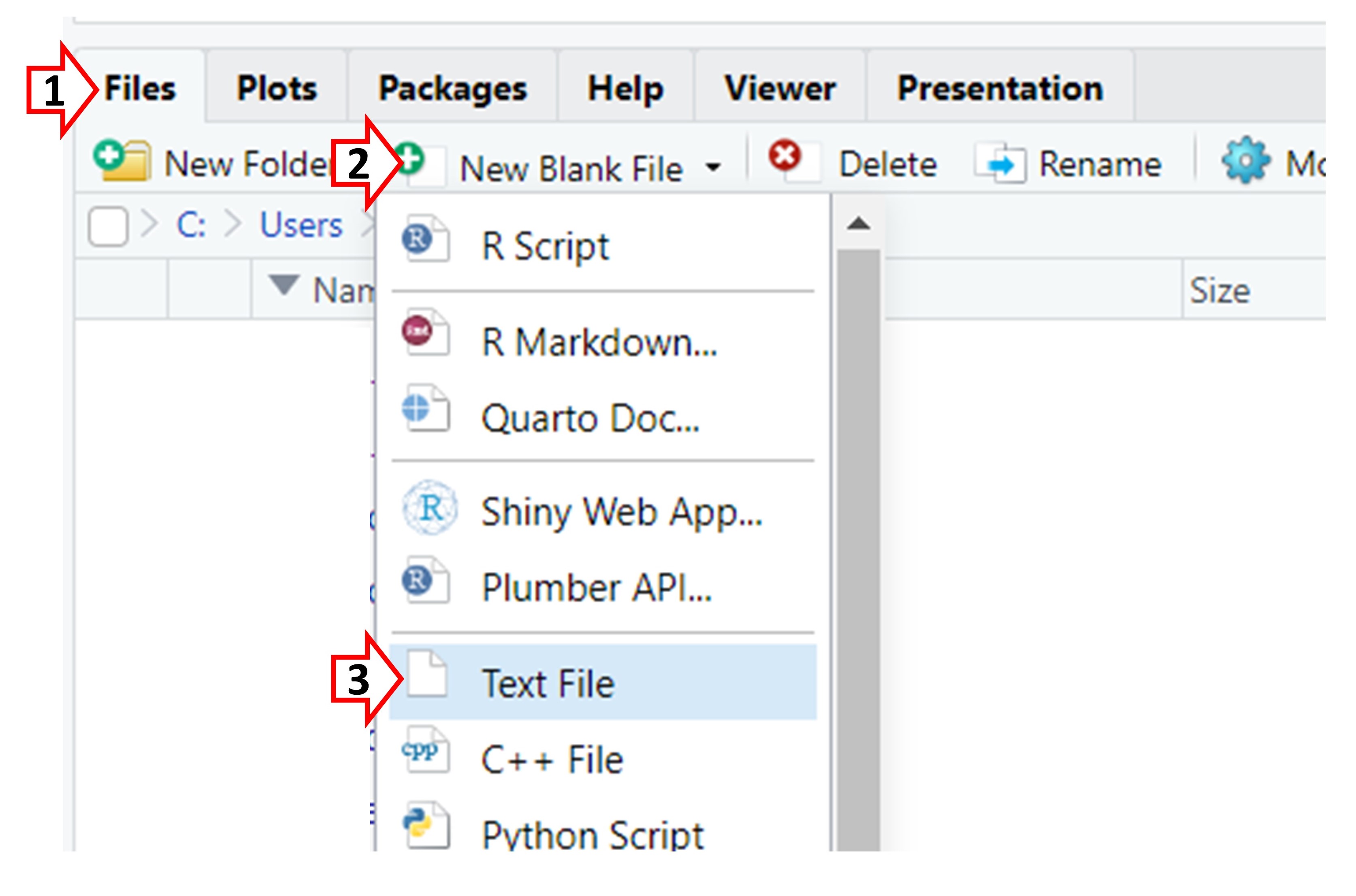
To get started, open RStudio and create a Quarto Document:

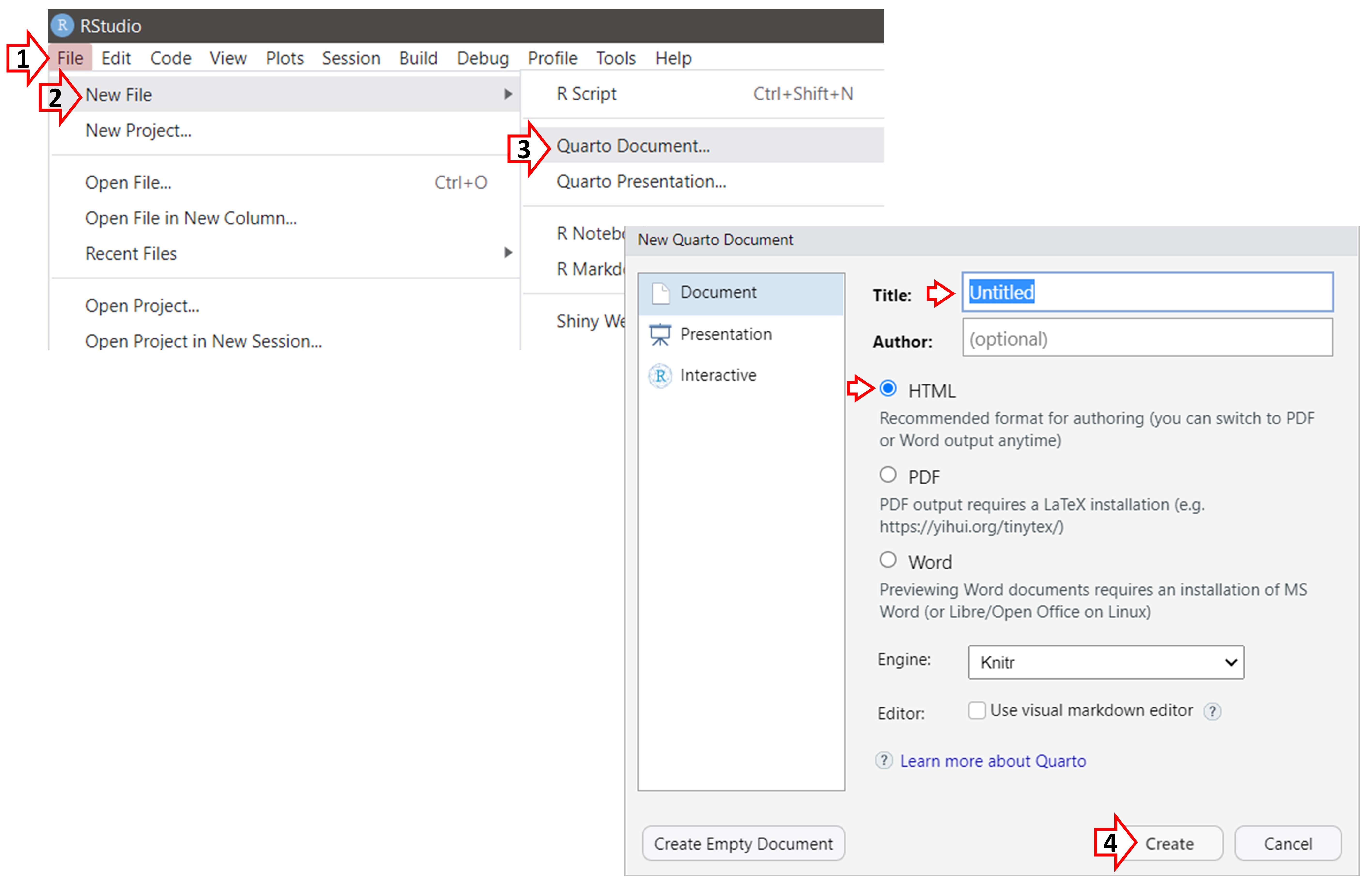
This will create a file with temporary content to help get you started.

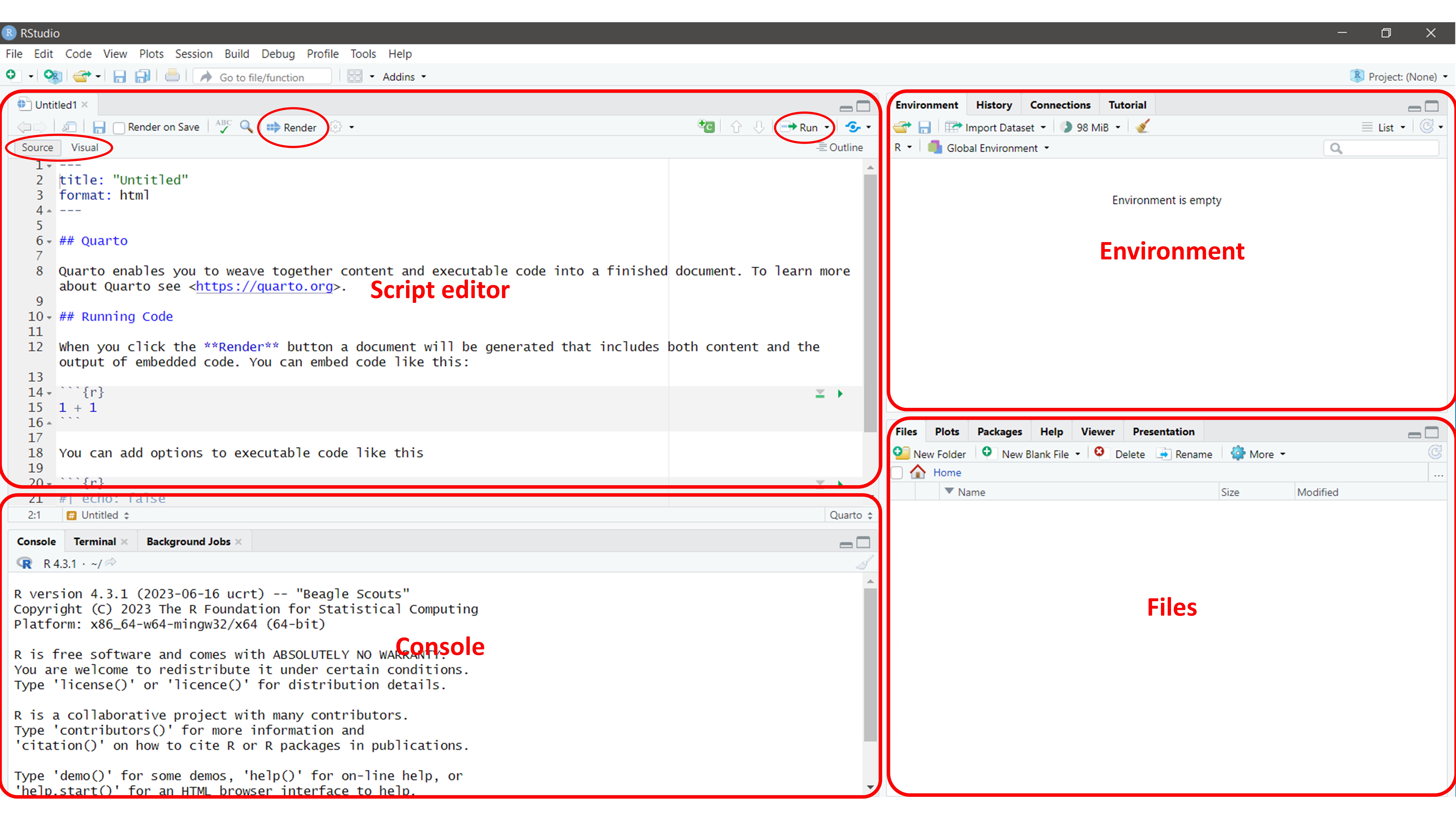
The script editor is where you write and edit your content. You can view the content using the Source view, which uses the raw syntax (used throughout this tutorial), or use the Visual view, which uses a point and click interface for formatting (similar to Microsoft Word).

All of the scripts provided below in this tutorial should be entered into the ‘Script Editor’. Clicking Render will generate the formatted document. You can also highlight code and click Run to execute specific lines of code.

The console is where you see the output of any statistical code. The environment panel displays information about the variables and objects in your current R session, while the files panel allows you to navigate your computer’s file system and manage your R projects.

3 Output Settings

Each quarto file starts with a set of code, called the YAML which is fenced within ---. The YAML specifics the metadata and document-wide settings. For example, for a HTML document the YAML may be:

Syntax (Input)

---
title: Introduction to Quarto
subtitle: My subtitle
author: Klajdi Puka
date: last-modified
format: 
  html:
    self-contained: true
execute:
  echo: true
  warning: false
toc: true
number-sections: true
editor_options: 
  chunk_output_type: console
---

Explanation

format specifies the type of output file to generate. Here it is an HTML file.

self-contained: true specifies that the HTML file generated should be standalone file.

echo: true enables the printing of code (only output is displayed), unless otherwise specified.

warning: false disables the printing of warning messages.

toc: true specifies that the table of contents should be shown; automatically generated based on the headings.

chunk_output_type: console specifies that when executing the code in RStudio (i.e., when you “run” the code, instead of “render”), the outcput in RStudio should be displayed in the “console” (where it typically appears when using R)

4 Formatting Basics

The following syntax works with Quarto and its predecessor Markdown. In addition to this code, RStudio has a ‘visual’ editor which provides a point-and-click interface to format the document.

Syntax (Input)


# Heading 1


## Heading 2

### Heading 3




Bold text like **this** or __this__

Italicize text like *this* or _this_




Clickable link: <https://google.com>

[Hyperlink](google.com) 



-   Bullet point (nordered lists)
-   Hyphen, follwed by 'tab'

1.    Ordered list
2.    Number, period, then 'tab'




|            | Manual   | Table    |
|------------|----------|----------|
| Variable 1 | 11       | 21       |
| Variable 2 | 12       | 22       |
| Variable 3 | 12       | 23       |

Formatted Output

Heading 1

Heading 2

Heading 3

Bold text like this or this

Italicize text like this or this

Clickable link: https://google.com

Hyperlink

Bullet point (nordered lists)
Hyphen, followed by ‘tab’

Ordered list
Number, period, then ‘tab’

	Manual	Table
Variable 1	11	21
Variable 2	12	22
Variable 3	12	23

To get properly formatted tables, using an online table generator may be helpful, such as this webpage..

5 Organization

5.1 Columns

To create and work with columns, use ::: or ::::. Like brackets, these are used to indicate the start and end the content to be placed in columns.

Here’s an example:

Quarto Syntax (Input)

:::: columns
::: {.column}
Content of column 1
:::

::: {.column}
Content of column 2
:::
::::

Explanation

:::: columns indicates that what comes next should be presented in columns.

::: {.column} indicates that what comes next are the content of column 1.

::: indicates the end of the content of column 1

The very last :::: indicates the end of the columns.

Additional arguments can be added within the curly brackets:

::: {.column width="40%"} indicates that the column should take up 40% of the screen
::: {.column font-size: "60%"} indicates that the content within the column should be a different size font
::: {.column .fragment} (for presentations) indicates that the content of the column should appear after a click
Multiple arguments can be integrated together: ::: {.column width="40%; font-size: 60%;" .fragment}

Most of this document is created using columns, such that the code is specified but not run in column 1, and in column 2 the code is repeated and implemented.

5.2 Layouts

Similar to columns, custom ‘layouts’ can also be used to create columns or a more complex organization of the output.

To create two columns, each taking up 50% of the page, you can use either one of the following:

Specify number of equally-sized columns

:::: {layout-ncol=2}
::: {#first-column}
Content of column 1
:::
    
::: {#Second-column}
Content of column 2
:::
::::

Manually specify proportion of each column

:::: {layout="[50, 50]"}
::: {#first-column}
Content of column 1
:::
    
::: {#Second-column}
Content of column 2
:::
::::

The id attributes (#first-column and #second-column) are optional, but aid readability.

Layouts are powerful because they can create complex organizations; for example:

:::: {layout="[[45, -10, 45], [100]]"}
:::{#Output1}
Content 1
:::

:::{#Output2}
Content 2
:::
        
:::{#Output3}
Content 2
:::
::::

This example will organize the three pieces of output in the following ways:

Output1 will show in the first row and take up 45% of the page width
Output2 will show in the first row and take up 45% of the page width
The -10 defined the amount of empty space between Output1 and Output2
Output3 will show in the second row, and take up 100% of the page width

Notably, these layout options can also be integrated within the code chunk. For example:


#| layout-ncol: 2

#| layout: [50, 50]

5.3 Callout Blocks

Callouts are used to draw extra attention to certain concepts, or to more clearly indicate that certain content is supplemental or applicable to only some scenarios.

Callouts start with ::: {.callout-note}, then there’s the content, and it ends with :::.

There are five types of callouts: note, warning, important, tip, and caution.

Quarto Syntax (Input)


:::{.callout-note}
This is a callout block of the type "note".
:::

:::{.callout-caution collapse="true"}
Callouts can be collapsible. 
:::

:::{.callout-important}
# My heading
The first heading used within the callout 
is used as the callout heading.
:::

:::{.callout-tip icon=false}
The icon can also be hidden, like this. 
:::


:::{.callout}
This is a simpler callout, without 
specifying the "type". 
:::

Formatted Output

Note

This is a callout block of the type “note”.

Danger

Callouts can be collapsible.

My heading

The first heading used within the callout is used as the callout heading.

Tip

The icon can also be hidden, like this.

This is a simpler callout, without specifying the “type”.

An alternative method of collapsing sections is presented in Section 8.5.2 and uses HTML code.

5.4 Tabsets

Another way to organize a report is to present information in different tabs.

Similarly, as before, this is coded using ::: to denote the start and end of the information to be presented in tabs.

Level 3 headings (specified using ###) are used as the tab title and denote the start of each new tab.

Here a simple example:

Syntax (Input)

::: {.panel-tabset}

### Panel 1 Title
Content of panel 1

### Panel 2 Title
Content of panel 2

:::

Content of panel 1

Content of panel 2

6 Integrating Statistical Code

Quarto can understand and run different programming languages, such as R and Python. This introduction focuses on R.

Code is specified within “code chunks”, which begin with ```{r} and end with ```

As an example, here’s a simple calculation using R; the syntax is shown along with the output automatically generated.

```{r}
1 + 1
```

[1] 2

6.1 Execution Options

There are a variety of options for how to handle the code and its output, called ‘execution options’. These options are specified at the start of the code chunk, and begin with #|

For example, to output just the code chunk, without executing the code and to ignore any warnings:

```{r}
#| eval: false
#| warning: false
1 + 1
```

Other execution options include:

eval: true indicates that the code chunk should be ‘evaluated’ or ‘run’
echo: true indicates the code chunk should be ‘echoed’ or shown along in the output
warning: false indicates that any warning messags should not be shown in the output
output: asis indicates that the output is raw markdown and should not have any of Quarto’s standard enclosing markdown
include: false is a catch all, indicating neither the code chunk nor results should be shown in the output
file: "Name of R file.R" can be used to import, display, and run the code that is in a separate file called “Name of R file.R”. Useful if you have custom functinos saved in a separate R script, and want to show the function code in your final document.
code-fold: true indicates that the code chunk is shown, but presented in a collapseble format
- #| code-summary: "Title of folding code" indicates the name used as the heading for the folding code

Example of a folded code:

Example of code fold

```{r}
#| code-fold: true
#| code-summary: "Example of code fold"
1 + 1
```

[1] 2

6.2 Formating the Report and Results

Any text (outside of code chunks) is automatically formatted by Quarto. To present nicely formatted tables and figures, a variety of packages are available. This includes the gt and gtsummary packages for tables, and the ggplot package for figures.

To present executable code inline with your text, enclose the expression in `r `. For example:

The sum of 1 + 1 is equal to `r 1+1`.

The sum of 1 + 1 is equal to 2.

6.3 Example of Analyses and Report

Syntax + Output
Output Only

```{r}
#| warning: false

# Load libraries and data.
library(tidyverse)       # Data management
library(gt)              # Create nicely formatted tables
library(gtsummary)       # Create summary tables
library(palmerpenguins)  # Contains the dataframe called "penguins"


# Lets calculate some numbers to be used later on
n_Adelie    <- filter(penguins, species=="Adelie") %>% nrow()
n_Chinstrap <- filter(penguins, species=="Chinstrap") %>% nrow()
n_Gentoo    <- filter(penguins, species=="Gentoo") %>% nrow()
```

Our data is comprised of `r nrow(penguins)` peguins; specifically comprised of the
species Adelie (n=`r n_Adelie`), Chinstrap (n=`r n_Chinstrap`), and Gentoo 
(n=`r n_Chinstrap`). Penguin charactersitics are presented in @tbl-demographics.

Our data is comprised of 344 peguins; specifically comprised of the species Adelie (n=152), Chinstrap (n=68), and Gentoo (n=68). Penguin charactersitics are presented in Table 1.

```{r}
#| label: tbl-demographics
#| tbl-cap: Penguin charactertics

penguins %>% 
  select(species, sex, flipper_length_mm, body_mass_g) %>%
  tbl_summary(
      by=species,
      missing = "no",
      statistic = list(all_continuous() ~ "{mean} ({sd})",
                       all_categorical() ~ "{n} ({p}%)"))
```

Table 1: Penguin charactertics
Characteristic	Adelie, N = 152¹	Chinstrap, N = 68¹	Gentoo, N = 124¹
sex
female	73 (50%)	34 (50%)	58 (49%)
male	73 (50%)	34 (50%)	61 (51%)
flipper_length_mm	190 (7)	196 (7)	217 (6)
body_mass_g	3,701 (459)	3,733 (384)	5,076 (504)
¹ n (%); Mean (SD)

Our analyses show that flipper length and body mass are related, see @fig-scatter.

Our analyses show that flipper length and body mass are related, see Figure 1.

```{r}
#| label: fig-scatter
#| fig-cap: Flipper length by body mass
#| fig-height: 4

ggplot(data = penguins, 
                       aes(x = flipper_length_mm,
                           y = body_mass_g)) +
  geom_point(aes(color = species, 
                 shape = species),
             size = 3,
             alpha = 0.8) +
  scale_color_manual(values = c("darkorange","purple","cyan4")) +
  labs(x = "Flipper length (mm)",
       y = "Body mass (g)",
       color = "Penguin species",
       shape = "Penguin species") +
  theme_minimal() + 
  theme(legend.position = c(0.2, 0.7),
        plot.title.position = "plot",
        plot.caption = element_text(hjust = 0, face= "italic"),
        plot.caption.position = "plot")
```

Warning: Removed 2 rows containing missing values (`geom_point()`).

Our data is comprised of 344 peguins; specifically comprised of the species Adelie (n=152), Chinstrap (n=68), and Gentoo (n=68). Penguin charactersitics are presented in Table 1.

Table 2: Penguin charactertics
Characteristic	Adelie, N = 152¹	Chinstrap, N = 68¹	Gentoo, N = 124¹
sex
female	73 (50%)	34 (50%)	58 (49%)
male	73 (50%)	34 (50%)	61 (51%)
flipper_length_mm	190 (7)	196 (7)	217 (6)
body_mass_g	3,701 (459)	3,733 (384)	5,076 (504)
¹ n (%); Mean (SD)

Our analyses show that flipper length and body mass are related, see Figure 1.

Warning: Removed 2 rows containing missing values (`geom_point()`).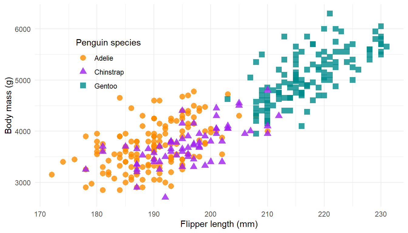

7 Parameterized Reports

Multiple versions of a document, using different settings or data subsets, can also be created with Quarto (and R Markdown) without duplicating the entire document. These are parameterized reports.

To begin, you need to define the parameters you want to use in the YAML using the params keyword. For example, let’s define a parameter called species with a default value of “Adelie”:

---
title: Parameterized report
format: html
params:
  species: Adelie
---

Once you have defined the parameters, you can use them throughout your document to make it dynamic. Parameters can be accessed using the params object within code chunks or inline expressions.

For instance, let’s say you have a code chunk that filters a dataset based on the selected species. You can use the params$species expression to access the value of the species parameter within the code chunk:

library(tidyverse)
library(palmerpenguins)

data <- penguins %>%
  filter(species == params$species)

# continue with rest of your code

To generate a different version of the report, you can change the specicies in the YAML and re-render the report.

You can also automate the process. In a separete Quarto file, you can code the following to 1) select the quarto file that contains your report, 2) change the paratemeters, and 3) save a separate report for each value of the parameter:

install.packages("quarto")
library(quarto)

my_function <- function(penguin){
  quarto_render(input = "Your_Quarto_file.qmd",
                execute_params = list(specifies=penguin),
                output_file = glue::glue("{penguin}-report.html"))
}

distinct(penguins, as.character(species)) %>% 
  pull () %>%
  purr:walk(my_function)

For more details on this approach and example, click here.

8 HTML Theming

8.1 HTML Basics

Quarto also support HTML, allowing for greater flexibility in formatting the final document. To use HTML, use triangle brackets: < and >; the formatting specified will be applied to the rest of the document, or until the code is ‘turned off’ by using the /.

Common HTML tags include:

Tag	Description
`<h1>` to `<h6>`	Headings of different levels
`<br>`	Line break
`<b>`	Bold text
`<i>`	Italic text
`<div>`	Section or container
`<span>`	Inline styling or grouping of elements
`<a>`	Hyperlink
`<form>`	Form container
`<style>`	CSS style declaration
`<script>`	JavaScript code

For example:

This is how you <b>bold</b> or <i>italicize</i> words.

This is how you bold or italicize words.

Similarly, you can use HTML’s <div> tag to create custom sections or containers with specific styles:

<div class="my_custom-section">
This is a custom section with a specific style (specified below).
</div>
  
This section defaults back to the original formatting.

This is a custom section with a specific style (specified below).

This section defaults back to the original formatting.

8.2 CSS Basics

HTML becomes even more powerful when you combine it with CSS (Cascading Style Sheets). CSS allows you to define styles and apply them to HTML elements, giving you full control over the document’s visual presentation. You can include CSS styles within your Quarto document using HTML’s <style> tag:

<style>
    .my_custom-section {
        background-color: #e32424;
        color: white;
        padding: 10px;
    }
</style>

In this example, we define a CSS style for the .my_custom-section class, specifying a background color, font color, and padding. This style will be applied to any <div> element with the my_custom-section class in your document.

By combining HTML and CSS, you can achieve a highly customized and visually appealing document layout.

8.3 Pre-set Themes

There are a number of pre-specified themes available, and can be specified in the YAML.

For example:

---
title: My Report
format:
  html:
    theme: cerulean
---

Quarto uses Bootstrap themes, with details available here. There you can also examine the preset formatting of various types of objects and utilize it in your Quarto document.

For example:

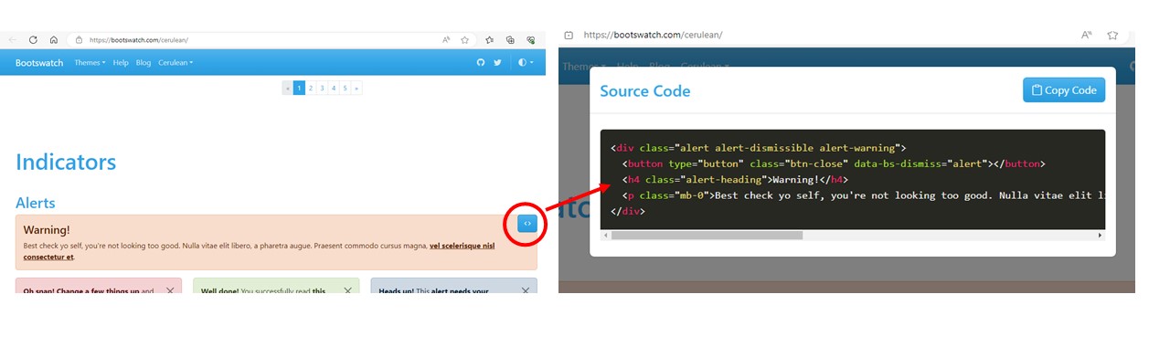
<div class="alert alert-warning">
  <h4 class="alert-heading">Heading</h4>
  Your text here.
</div>

Heading

Your text here.

8.4 Custom Themes

To create a custom theme or modify an existing, you will need to create a text file with an ending of “.scss”; this file will list your specifications.

SASS: Syntactically Awesome Style Sheets

SASS files have the “.scss” extension. These files extend the functionality of CSS by allowing for a more organized and modular stylesheets, making it easier to manage and maintain your styles.

Create the ‘.scss’ file by creating a new text file while still in RStudio; here we name it ‘mytheme.scss’:

Reference the file created in the YAML of your Quarto document; multiple theme files can be used:

---
title: My Report
format:
  html:
    theme: 
      - cerulean
      - mytheme.scss
---

To specify your theme, open the SASS file and list the specifications. Importantly, the file should begin with /*-- scss:defaults --*/. Here’s an example:


/*-- scss:defaults --*/

$blue: #1F3169;

.my_custom-section2 {
    background-color: $blue;
    color: white;
    padding: 10px;
}

The advantage of SASS over CSS is that we can define colors or settings, to be used later. In the example above, we have assigned hex color #1F3169 the variable label of blue; this label can then be referred to in other sections of the code. In this example, we are using CSS to create a new class (like we did earlier), but here we specify the color as blue.

This becomes more powerful when combined with the pre-specified themes and settings of Quarto. Quarto has predefined SASS variables that can be changed and modified to adjust the appearance of your report. The available variables can be found here. If the variables listed there are not enough, the complete list can be found here; use the search function to identify variables that seem like they may change the feature you are interested in.

Once you have idenfied the variable, you can specify the value; the general form is: $variable_name: value;. Comments begin with a //.

For example:


/*-- scss:defaults --*/

// Color of the text in the body of the document.
$body-color: #000000;
  
// Page background color.
$body-bg: #fff;
  
// Font size (reference is 1rem).
$font-size-base: 1.2rem;

8.5 Other Formatting Examples

8.5.1 Watermmark

To add a watermark to a HTML document, you can use CSS code, like so:

<style>
.draft-watermark {
    position: fixed; top: 50%; left: 50%;
    transform: translate(-50%, -50%) rotate(-45deg);
    font-size: 100px; font-weight: bold; color: #ccc; opacity: 0.5; }
</style>

<div class="draft-watermark">Draft</div>

The first part, enclosed within the <style> and </style> lists the details of the watermark.

The second part, enclosed within the <div> and </div> applies the settings specified.

8.5.2 Collapsible Sections

Although you can use ‘callouts’ to highlight or collapse sections, if you do not want the formatting that is associated with callouts, you can use HTML code.

<details>
<summary> Title here</summary>
Details go here. This will be collapsed. 
</details>

Title here

Details go here. This will be collapsed.

8.6 Troubleshooting

If something is not working but it should, you may just need to ensure that there is an empty line before/after the HTML tag.

9 Additional Resources

Quarto’s comprehensive guidance documentation: https://quarto.org.

Introduction to Quarto: https://www.youtube.com/watch?v=_f3latmOhew&ab_channel=PositPBC

Quarto for academics: https://www.youtube.com/watch?v=EbAAmrB0luA&t=669s&ab_channel=PositPBC

HTML and CSS formatting: https://ucsb-meds.github.io/customizing-quarto-websites/#/title-slide

Quarto blogs: https://albert-rapp.de/posts/13_quarto_blog_writing_guide/13_quarto_blog_writing_guide.html

Quarto website: https://ucsb-meds.github.io/creating-quarto-websites/