Regressions 1: Linear Regression
Topic: Introduction to linear regression, interpretation of results, assumptions, and the selection of variables.
Introduction
Linear regression is a method of describing the relationship between a continuous outcome variable (Y) and one or more ‘predictor’ variable(s) (X) that can be binary, categorical, or continuous. Other forms of regression are used when the outcome is binary (logistic regression), categorical (multinomial regression), ordinal (ordinal regression), count data (Poisson regression), or time-to-event data (Cox Models).
How is it Calculated, and What Do Those Numbers Mean?
The figure below shows a scatter plot of two continuous variables (X and Y). We can describe the relationship between X and Y by drawing a straight line through the data points. The data points represent the observed values, whereas the line represents the predicted values; the difference between these two is called the “error” or a “residual”. The line drawn is as close as possible to the data points, specifically, the line of best fit is the one that has the smallest value for the sum of all the “errors” or “residuals”.
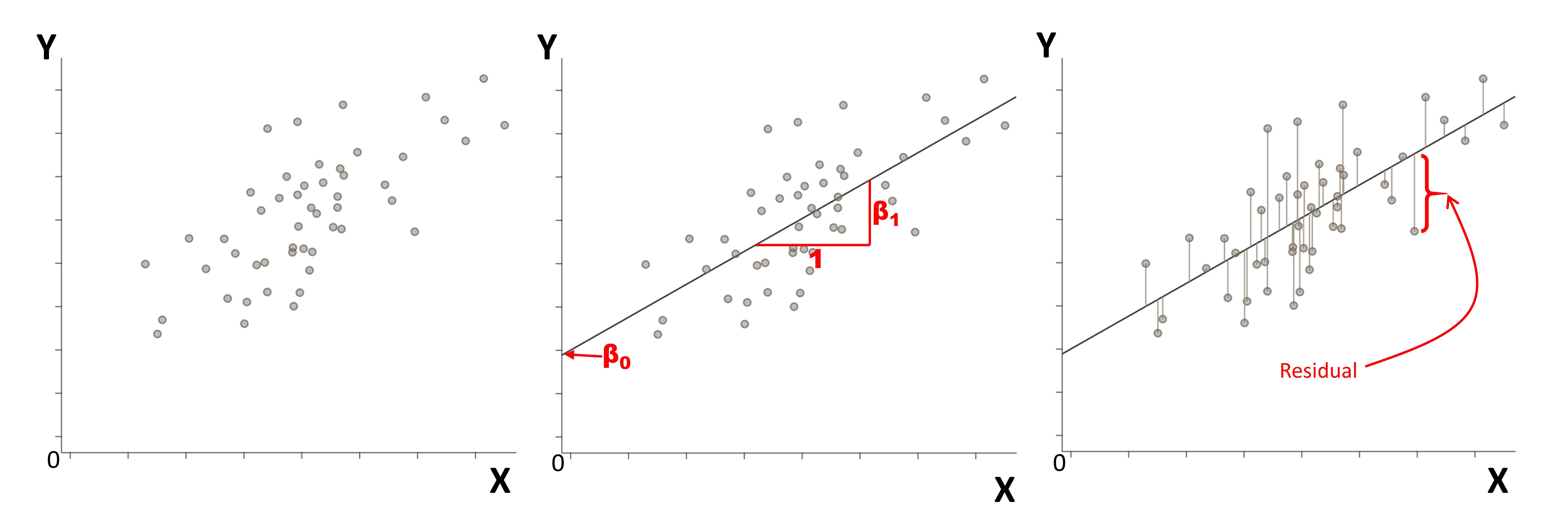
The line may be described by the equation:
\[ Y = (intercept)+(slope)(X) = β_0 + (β_1)(X) \]
The intercept (β0) is the estimated Y when X = 0.
The slope (β1) is the estimated change in Y for a one-unit increase in X.
With this equation, we can estimate the value of Y for any given value of X.
The value of β0 and β1 are calculated and are of key interest when conducting a regression. The null-hypothesis is that the regression coefficients (i.e., β0 and β1) equal to 0, that is, the p-values associated with β0 and β1 indicate whether they are different from 0. If the line has a slope of zero (i.e., a flat horizontal line; β1 = 0), X and Y are not associated with each other; the expected value of Y will be the same regardless of the value of X.
When there are two predictors (X1 and X2), the regression equation becomes:
\[ Y = β_0 + (β_1)(X_1) + (β_2)(X_2) \]
β0 is the estimate of Y when X1=0 and X2=0.
β1 = expected change in Y for a one unit increase in X1 and all other variables (e.g. X2) stay the same.
β2 = expected change in Y for a one unit increase in X2 and all other variables (e.g. X1) stay the same.
β values represent the independent effect of the predictor on the outcome ‘controlling for’, ‘adjusted for’, or ‘holding constant’ all other variables.
This model can be expanded to include many predictors:
\[ Y = β_0 + (β_1)(X_1) + (β_2)(X_2) + (β_3)(X_3) +... + (β_n)(X_n)\]
Assumptions
- Linearity – relationship between the outcome (Y) and the covariates (X) is linear
- Independence – observations/participants are independent of each other
- Normality – the residuals (not the outcome) are normally distributed
- Homogeneity of variance – the residuals have a constant variance across the levels of X (that is, the variability around the regression line is constant/similar throughout the regression line).
Additionally, you should avoid including covariates that are highly correlated in the same regression model (this is because it becomes much harder to identify their independent effects; this issue is called multicollinearity). Outliers may also be a concern and may skew results – observations with large residuals may need to be removed or a different model needs to be used.
Note that there are no assumptions about the distribution of the covariates (X).
Categorical Predictors
The interpretations discussed above expand to binary covariates, (e.g., variables with 2 categories, such as male vs. female). A linear regression with one binary covariate is equivalent to an independent samples t-test. If the variable is coded with a 0 and 1 (e.g., 0 = female, 1 = male), then:
β0 = estimate of Y when X = 0; i.e. the mean of the group coded 0. In our example, if β0 = 10.0, the mean score of females is 10.0.
β1 = estimated change of Y when there is a 1 unit increase in X; i.e. the difference in the mean outcome of the two groups. In our example, if β1 = 5.0, then mean score of males is 5.0 points higher than females. Since mean score of females is 10.0, the mean score of males is 15.0.
If the predictor has more than 2 categories, one of the categories is set as the ‘reference’ category, and other categories are compared against it, similar to above. The reference group is usually the largest group or most clinically relevant.
Selection of Variables to Enter in the Model
- A larger sample size is required when multiple predictors are added to the model
- Prior knowledge from the scientific literature is the most important rationale. Which variables are known or thought to affect the outcome you are studying?
- Do not remove variables just because they are not significant (p >.05). A p>.05 is not a sign that the variables do nothing, it just means that the effects of those variables could not be detected from the sample. Leaving in not-significant variables ensures that your confidence intervals and p-values have the correct interpretation, and they are the most faithful estimates you can make
- Avoid including variables which are largely homogenous between participants. For example, if you are studying 100 patients, and only 3 of them smoke, the effects of smoking may not be estimated very well due to the small sample of those participants
- Automated variable selection methods (backward/forward selection) provide biased results and should be avoided; they produce more extreme regression coefficients, and incorrect confidence intervals and p-values. These issues are outlined in Regression Modeling Strategies (Harrell, 2015), section 4.3, and also summarised here.
Comparing and Centering Regression Coefficients
In general, it is not possible to compare regression coefficients directly. This is because they describe the effects of a one-unit change in a variable (X), therefore, the magnitude of the regression coefficient is dependent on the units of the covariate.
To compare regression coefficients, they must be on the same scale. If the variables are in different scales, standardized regression coefficients (which range from -1 to +1) can be calculated/used. You can also express the effect of a change in one unit of predictor X2 as the number of units of predictor X1 giving the same effect – this is simply the ratio of the two regression coefficients: β2 / β1. For example, a ‘one hour of physical activity per week has the same effect as a difference of 2 years of age’.
Centering Covariates
β0 is the value of Y when all predictors equal zero; this value may not be meaningful (e.g. estimated running speed when blood pressure is equal to 0 is not a meaningful number). In such cases, you can redefine the 0 point to make β0 meaningful, if that is of interest to you. Can do so by ‘centering’ the covariate(s); that is, subtract a constant from every value of a variable. If that constant is the sample mean, the new variable will have a mean of 0. The intercept (β0) can be interpreted as the estimated Y for the ‘average participant’. Aadding or subtracting a constant from covariates (X1, X2, etc.) will change the value of β0 but not the other regression coefficients (β1, β2 , etc.). If variables are centered, this should be made clear in the publication.
References and Further Readings
Harrell F. Regression Modelling Strategies With Applications to Linear Models, Logistic and Ordinal Regression, and Survival Analysis. Springer. 2015
Werner V. Regression models as a tool in medical research. NY: Taylor & Francis Inc. 2012.