?meanIntroduction to R
Topic: Introduction to data wrangling and data management with R.
R is a powerful programming language and software environment widely used for statistical computing, data analysis, and graphical visualization.
Getting Started
To get started, you will need to install R and RStudio; to do so click here.
To use R, launch RStudio. RStudio provides a user-friendly interface for working with R.
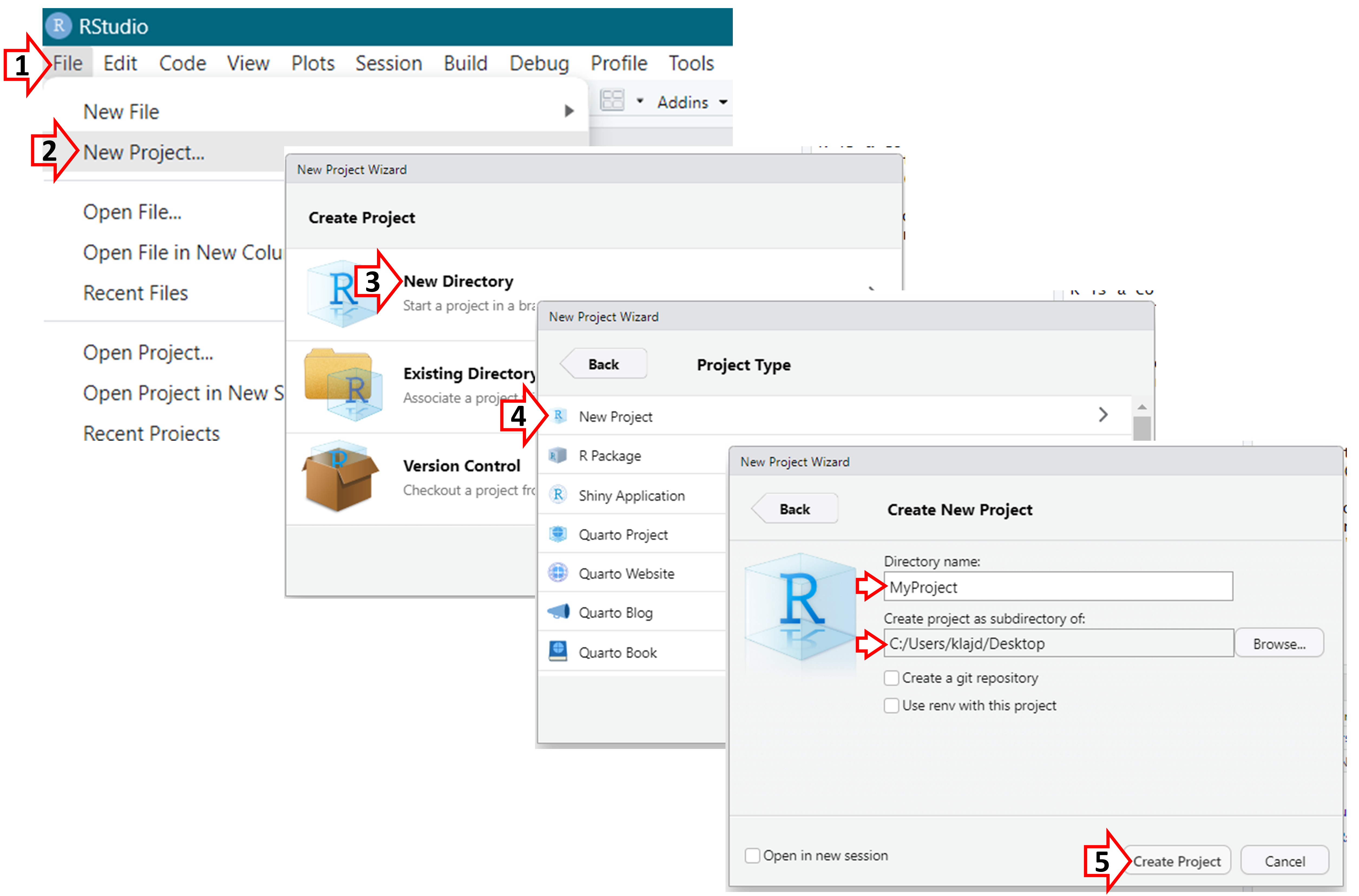
For each project, you should use “R Projects”, a self-contained directory that holds all the files, data, R scripts, and other resources related to a particular data analysis task or research project. Follow the steps below to create an R Project.
Important
Upon creating an ‘R Project’, a folder will be created in the location that was specified; this folder should contain all of the files needed for your analyses (e.g., the data and R code files).
In that folder, a “.Rproj” file will also be created (in this example, called “MyProject.Rproj”); this is the file you should open in the future when you want to work with your data in R.
Next, lets create an R script; this will be the file that will contain your R code. 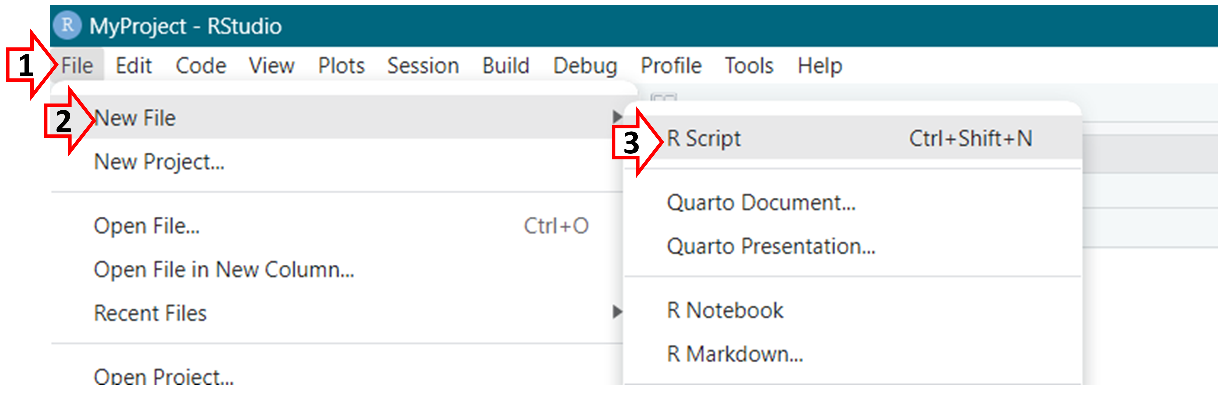
Now, lets examine RStudio and its different components. 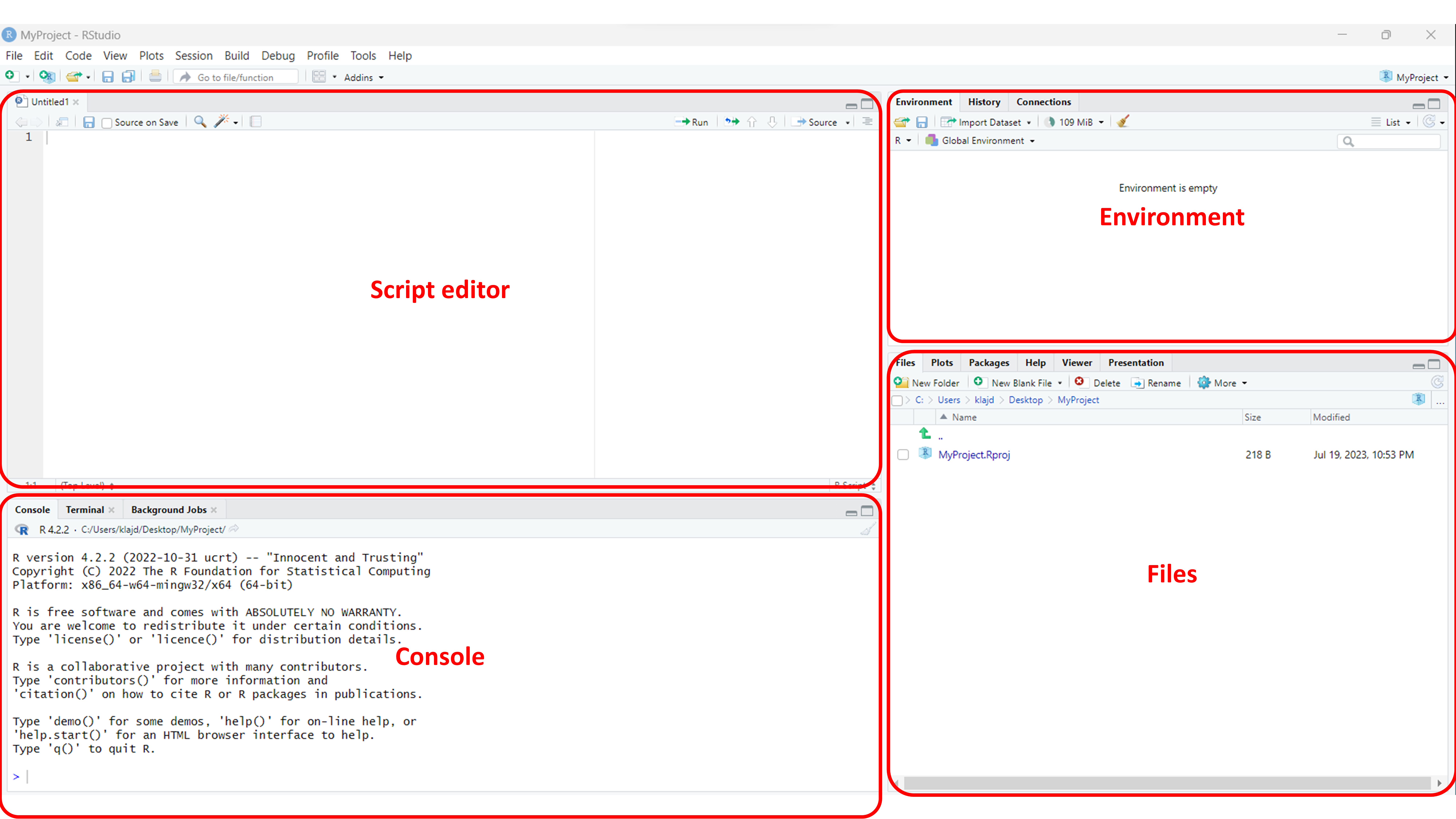
The script editor is where you write and edit your R code. The console is where you see the output of your commands and interact with R directly. The environment panel displays information about the variables and objects in your current R session, while the files panel allows you to navigate your computer’s file system and manage your R projects.
Important
All of the R code provided below in this tutorial should be entered into the ‘Script Editor’.
To run/execute the code, highlight the portion of code you would like to execute and press “Run” (located in the top right corner of the script editor). On Windows, you can also use the shortcut “Ctrl + Enter”.
R Basics
Functions and Packages
- Functions essential building blocks that enable you to perform specific tasks efficiently. They are like a set of instructions designed to carry out various operations, saving you from having to write complex code each time you want to perform a common task.
- In R, a function is a named block of code that takes inputs (arguments) and returns outputs (results).
- For example,
mean()calculates the mean of a set of numbers, so you don’t have to write the formula to calculate the mean each time
- Packages, just like smartphone apps, are created by individuals/groups and extend the functionality of R by providing a a collection of functions
- To use packages:
- First time only: install the package using
install.packages("package_name") - Each time you open R: load the package using
library(package_name)
- First time only: install the package using
- Sometimes, different packages may use the same function name
- To specify the package and function name:
package_name::function_name()
- To specify the package and function name:
- R’s vast collection of packages, combined with the ability to create your own functions, make it a powerful tool
Basic Operations and Functions
| Operator | Description |
|---|---|
| $ | Used to access/refer to specific elements/variables within a data frame or list |
| <- | “save as”. Arrow pointing to the left - the object on the left will be defined/crehtated based on the instructions on the right |
| |> %>% |
“and then”, will take the output from the first function and use it as the first input of the second function. For example: function(data, arguments) is the same as data |> function(arguments) |
| ( ) | Used primarily to specify the arguments of a function |
| c( ) | Is a function allowing you to combine multiple elements into a single object. It stands for ‘combine’ or ‘concatenate’ |
| | | Or |
| & | And |
Resources and Help Files
- Helpful books include R for Data Science and Advanced R
- Many packages also have websites, such as https://www.tidyverse.org/packages/
- Google, and more recently chatGPT, will be your best friend
- R has built-in help files that provide syntax, arguments, usage, and examples
- To access a help file, use
?followed by the function name (e.g.?mean)
- To access a help file, use
Today’s Data
Will be using publicly available data from the 2018 US National Health Interview Survey (NHIS).
- This is an annual, cross-sectional survey of the US population; full data and details available here
- We will use a subset of the data from the “Sample Adult Interview”:
- To download this data, click here
- To download the codebook, click here
TipData
| ID | REGION | AGE_P | SEX | R_MARITL | AHEIGHT | AWEIGHTP | ASISLEEP | HYPEV | CHLEV | DIBEV1 | AHSTATYR | SMKSTAT2 | ASISAD | ASINERV | ASIRSTLS | ASIHOPLS | ASIEFFRT | ASIWTHLS |
|---|---|---|---|---|---|---|---|---|---|---|---|---|---|---|---|---|---|---|
| 1 | 3 | 66 | 2 | 1 | 66 | 180 | 8 | 2 | 2 | 2 | 3 | 4 | 5 | 5 | 5 | 5 | 5 | 5 |
| 2 | 3 | 18 | 2 | 7 | 63 | 123 | 7 | 2 | 2 | 2 | 3 | 4 | 1 | 5 | 5 | 5 | 5 | 5 |
| 3 | 1 | 64 | 1 | 7 | 67 | 196 | 7 | 1 | 1 | 1 | 2 | 2 | 4 | 5 | 5 | 5 | 5 | 5 |
| 4 | 4 | 25 | 2 | 7 | 63 | 110 | 7 | 2 | 2 | 2 | 3 | 4 | 5 | 5 | 5 | 5 | 5 | 5 |
| 5 | 4 | 61 | 1 | 7 | 72 | 250 | 6 | 1 | 1 | 2 | 3 | 3 | 5 | 5 | 5 | 5 | 5 | 5 |
| 6 | 1 | 39 | 1 | 1 | 67 | 135 | 6 | 2 | 2 | 2 | 3 | 4 | 5 | 4 | 5 | 5 | 5 | 5 |
| 7 | 2 | 22 | 2 | 7 | 65 | 200 | 7 | 2 | 2 | 2 | 3 | 4 | 5 | 3 | 4 | 5 | 5 | 5 |
| 8 | 3 | 46 | 2 | 1 | 61 | 150 | 6 | 2 | 2 | 2 | 3 | 4 | 5 | 5 | 5 | 5 | 5 | 5 |
| 9 | 2 | 64 | 2 | 1 | 67 | 188 | 8 | 2 | 2 | 2 | 1 | 4 | 4 | 5 | 5 | 5 | 5 | 5 |
| 10 | 1 | 51 | 2 | 5 | 59 | 130 | 10 | 1 | 2 | 2 | 3 | 4 | 2 | 5 | 5 | 5 | 1 | 5 |
| 11 | 2 | 36 | 2 | 1 | 67 | 115 | 8 | 2 | 2 | 2 | 3 | 4 | 5 | 4 | 4 | 5 | 5 | 5 |
| 12 | 2 | 38 | 2 | 1 | 65 | 997 | 8 | 2 | 2 | 2 | 3 | 4 | 5 | 5 | 5 | 5 | 5 | 5 |
| 13 | 3 | 66 | 2 | 1 | 59 | 120 | 6 | 2 | 2 | 2 | 3 | 4 | 5 | 5 | 4 | 5 | 5 | 5 |
| 14 | 3 | 70 | 1 | 8 | 75 | 237 | 9 | 1 | 1 | 1 | 1 | 3 | 5 | 5 | 2 | 5 | 4 | 5 |
| 15 | 4 | 77 | 1 | 1 | 68 | 220 | 7 | 1 | 1 | 2 | 3 | 4 | 2 | 2 | 2 | 2 | 2 | 2 |
| 16 | 3 | 73 | 1 | 1 | 70 | 215 | 7 | 1 | 1 | 2 | 3 | 3 | 5 | 5 | 5 | 5 | 5 | 5 |
| 17 | 3 | 48 | 1 | 1 | 96 | 996 | 7 | 2 | 2 | 2 | 3 | 4 | 5 | 4 | 3 | 4 | 4 | 4 |
| 18 | 2 | 38 | 2 | 2 | 96 | 996 | 5 | 2 | 2 | 2 | 3 | 3 | 5 | 5 | 5 | 5 | 5 | 5 |
| 19 | 3 | 71 | 2 | 1 | 68 | 148 | 8 | 2 | 1 | 2 | 1 | 4 | 5 | 5 | 5 | 5 | 5 | 5 |
| 20 | 3 | 80 | 2 | 4 | 62 | 172 | 4 | 1 | 1 | 2 | 3 | 4 | 5 | 5 | 5 | 5 | 5 | 5 |
| 21 | 4 | 39 | 2 | 1 | 66 | 108 | 5 | 2 | 2 | 2 | 9 | 3 | 4 | 1 | 1 | 4 | 1 | 5 |
| 22 | 2 | 68 | 2 | 4 | 62 | 173 | 8 | 1 | 1 | 2 | 3 | 4 | 5 | 5 | 5 | 5 | 5 | 5 |
| 23 | 3 | 23 | 2 | 7 | 67 | 160 | 7 | 2 | 2 | 2 | 3 | 4 | 5 | 5 | 5 | 5 | 5 | 5 |
| 24 | 2 | 73 | 2 | 1 | 66 | 175 | 7 | 1 | 2 | 2 | 3 | 3 | 5 | 5 | 4 | 5 | 5 | 5 |
| 25 | 3 | 43 | 1 | 2 | 74 | 295 | 7 | 1 | 1 | 2 | 1 | 4 | 5 | 5 | 4 | 5 | 5 | 5 |
| 26 | 3 | 41 | 2 | 7 | 62 | 148 | 7 | 2 | 1 | 2 | 3 | 4 | 5 | 5 | 5 | 5 | 4 | 5 |
| 27 | 4 | 56 | 2 | 7 | 63 | 211 | 5 | 1 | 1 | 2 | 3 | 4 | 3 | 5 | 5 | 5 | 3 | 5 |
| 28 | 4 | 39 | 2 | 1 | 64 | 150 | 7 | 2 | 2 | 2 | 3 | 2 | 5 | 5 | 5 | 5 | 5 | 5 |
| 29 | 4 | 35 | 2 | 8 | 62 | 125 | 8 | 1 | 1 | 2 | 1 | 1 | 3 | 2 | 1 | 5 | 4 | 5 |
| 30 | 3 | 46 | 2 | 1 | 61 | 158 | 7 | 2 | 2 | 2 | 1 | 4 | 5 | 5 | 5 | 5 | 5 | 5 |
| 31 | 3 | 41 | 2 | 1 | 59 | 113 | 5 | 2 | 2 | 2 | 3 | 3 | 5 | 5 | 5 | 5 | 5 | 5 |
| 32 | 2 | 52 | 1 | 1 | 96 | 996 | 6 | 2 | 2 | 2 | 3 | 3 | 5 | 3 | 3 | 4 | 2 | 4 |
| 33 | 3 | 78 | 1 | 1 | 68 | 177 | 6 | 1 | 2 | 2 | 3 | 3 | 5 | 5 | 5 | 5 | 5 | 5 |
| 34 | 1 | 41 | 1 | 1 | 70 | 190 | 7 | 2 | 1 | 2 | 3 | 4 | 5 | 5 | 5 | 5 | 3 | 5 |
| 35 | 3 | 50 | 1 | 1 | 67 | 154 | 6 | 2 | 2 | 2 | 3 | 3 | 5 | 5 | 5 | 5 | 5 | 5 |
| 36 | 2 | 66 | 2 | 4 | 62 | 180 | 6 | 1 | 2 | 2 | 3 | 4 | 5 | 5 | 5 | 5 | 5 | 5 |
| 37 | 2 | 52 | 1 | 1 | 70 | 175 | 7 | 2 | 2 | 2 | 3 | 4 | 5 | 5 | 1 | 5 | 4 | 5 |
| 38 | 3 | 59 | 2 | 5 | 65 | 175 | 7 | 2 | 1 | 1 | 2 | 2 | 2 | 2 | 2 | 3 | 3 | 5 |
| 39 | 2 | 37 | 2 | 2 | 67 | 187 | 8 | 2 | 2 | 2 | 3 | 1 | 5 | 5 | 5 | 5 | 3 | 5 |
| 40 | 3 | 50 | 1 | 1 | 66 | 200 | 8 | 1 | 2 | 1 | 3 | 4 | 8 | 8 | 8 | 8 | 8 | 8 |
| 41 | 2 | 36 | 1 | 7 | 98 | 998 | 98 | 2 | 2 | 2 | 3 | 4 | 8 | 8 | 8 | 8 | 8 | 8 |
| 42 | 1 | 58 | 2 | 1 | 66 | 155 | 6 | 2 | 2 | 2 | 3 | 3 | 5 | 4 | 4 | 5 | 5 | 5 |
| 43 | 3 | 65 | 2 | 7 | 65 | 225 | 10 | 1 | 1 | 3 | 3 | 1 | 5 | 5 | 5 | 5 | 5 | 5 |
| 44 | 1 | 43 | 1 | 1 | 76 | 180 | 7 | 2 | 2 | 2 | 3 | 1 | 5 | 5 | 5 | 5 | 5 | 5 |
| 45 | 1 | 56 | 1 | 5 | 64 | 192 | 6 | 2 | 2 | 2 | 3 | 3 | 5 | 5 | 5 | 5 | 5 | 5 |
| 46 | 3 | 59 | 1 | 1 | 70 | 275 | 8 | 2 | 2 | 2 | 3 | 4 | 4 | 5 | 5 | 5 | 3 | 5 |
| 47 | 3 | 44 | 1 | 1 | 71 | 210 | 7 | 1 | 1 | 2 | 3 | 4 | 5 | 4 | 5 | 5 | 4 | 5 |
| 48 | 3 | 36 | 2 | 4 | 63 | 250 | 6 | 1 | 2 | 2 | 3 | 4 | 5 | 5 | 5 | 5 | 4 | 5 |
| 49 | 3 | 47 | 1 | 1 | 67 | 210 | 6 | 1 | 2 | 2 | 3 | 4 | 5 | 5 | 5 | 5 | 5 | 5 |
| 50 | 4 | 73 | 1 | 7 | 71 | 165 | 9 | 2 | 1 | 2 | 3 | 3 | 5 | 5 | 5 | 5 | 5 | 5 |
| 51 | 3 | 71 | 1 | 6 | 66 | 127 | 10 | 1 | 1 | 2 | 3 | 4 | 5 | 5 | 5 | 5 | 5 | 5 |
| 52 | 2 | 27 | 1 | 7 | 69 | 130 | 6 | 2 | 2 | 2 | 1 | 4 | 3 | 3 | 3 | 5 | 5 | 5 |
| 53 | 1 | 71 | 1 | 5 | 67 | 185 | 7 | 2 | 2 | 2 | 3 | 3 | 3 | 4 | 3 | 3 | 3 | 5 |
| 54 | 3 | 71 | 2 | 4 | 65 | 180 | 7 | 1 | 1 | 1 | 3 | 3 | 5 | 1 | 3 | 5 | 5 | 5 |
| 55 | 3 | 52 | 1 | 1 | 75 | 240 | 6 | 1 | 1 | 2 | 3 | 4 | 4 | 5 | 3 | 5 | 4 | 5 |
| 56 | 4 | 44 | 2 | 7 | 62 | 999 | 98 | 2 | 2 | 2 | 3 | 4 | 8 | 8 | 8 | 8 | 8 | 8 |
| 57 | 2 | 36 | 2 | 7 | 68 | 185 | 99 | 2 | 2 | 2 | 3 | 4 | 5 | 4 | 5 | 5 | 5 | 5 |
| 58 | 3 | 24 | 2 | 1 | 65 | 160 | 6 | 2 | 2 | 2 | 3 | 4 | 5 | 5 | 5 | 5 | 5 | 5 |
| 59 | 3 | 64 | 1 | 7 | 71 | 235 | 6 | 1 | 1 | 1 | 3 | 3 | 5 | 5 | 5 | 5 | 5 | 5 |
| 60 | 3 | 75 | 2 | 4 | 65 | 999 | 8 | 1 | 1 | 1 | 2 | 4 | 1 | 2 | 2 | 2 | 2 | 2 |
| 61 | 3 | 20 | 1 | 7 | 73 | 160 | 7 | 2 | 1 | 2 | 1 | 4 | 5 | 5 | 5 | 5 | 1 | 5 |
| 62 | 3 | 78 | 2 | 4 | 64 | 180 | 5 | 1 | 1 | 2 | 3 | 4 | 3 | 5 | 3 | 3 | 3 | 3 |
| 63 | 3 | 53 | 1 | 1 | 65 | 240 | 5 | 1 | 1 | 3 | 3 | 4 | 2 | 2 | 2 | 2 | 2 | 5 |
| 64 | 3 | 46 | 2 | 1 | 66 | 152 | 7 | 1 | 2 | 2 | 1 | 4 | 5 | 5 | 5 | 5 | 5 | 5 |
| 65 | 1 | 77 | 2 | 4 | 59 | 160 | 11 | 1 | 2 | 2 | 1 | 3 | 5 | 5 | 5 | 5 | 5 | 5 |
| 66 | 2 | 37 | 1 | 8 | 75 | 149 | 7 | 2 | 2 | 2 | 2 | 2 | 5 | 5 | 4 | 5 | 5 | 5 |
| 67 | 4 | 24 | 2 | 7 | 64 | 170 | 7 | 2 | 2 | 2 | 3 | 4 | 5 | 5 | 5 | 5 | 5 | 5 |
| 68 | 2 | 33 | 2 | 1 | 62 | 210 | 7 | 2 | 2 | 2 | 1 | 4 | 5 | 4 | 5 | 5 | 4 | 5 |
| 69 | 3 | 79 | 1 | 5 | 68 | 186 | 6 | 1 | 1 | 1 | 3 | 4 | 3 | 5 | 5 | 5 | 5 | 5 |
| 70 | 4 | 22 | 2 | 7 | 65 | 120 | 7 | 2 | 2 | 2 | 3 | 4 | 5 | 5 | 5 | 5 | 4 | 5 |
| 71 | 4 | 47 | 2 | 8 | 64 | 170 | 7 | 2 | 2 | 2 | 3 | 4 | 1 | 5 | 5 | 5 | 5 | 3 |
| 72 | 3 | 64 | 1 | 1 | 65 | 224 | 6 | 1 | 1 | 1 | 3 | 3 | 5 | 3 | 2 | 5 | 3 | 5 |
| 73 | 3 | 55 | 2 | 4 | 96 | 996 | 7 | 1 | 2 | 2 | 2 | 1 | 1 | 1 | 1 | 1 | 1 | 1 |
| 74 | 3 | 59 | 2 | 7 | 97 | 997 | 98 | 1 | 2 | 2 | 3 | 1 | 8 | 8 | 8 | 8 | 8 | 8 |
| 75 | 3 | 51 | 2 | 1 | 63 | 125 | 8 | 2 | 2 | 2 | 3 | 4 | 5 | 4 | 5 | 5 | 5 | 5 |
| 76 | 3 | 44 | 2 | 1 | 63 | 201 | 8 | 2 | 2 | 2 | 1 | 4 | 4 | 4 | 4 | 4 | 4 | 5 |
| 77 | 3 | 83 | 2 | 5 | 67 | 999 | 8 | 2 | 2 | 2 | 2 | 3 | 5 | 5 | 5 | 5 | 5 | 5 |
| 78 | 2 | 19 | 1 | 7 | 71 | 255 | 9 | 1 | 2 | 2 | 1 | 4 | 5 | 5 | 4 | 5 | 5 | 5 |
| 79 | 4 | 30 | 1 | 1 | 72 | 175 | 5 | 2 | 2 | 2 | 3 | 1 | 3 | 3 | 3 | 3 | 3 | 3 |
| 80 | 3 | 57 | 1 | 1 | 74 | 230 | 10 | 1 | 1 | 1 | 3 | 3 | 5 | 5 | 5 | 5 | 5 | 5 |
| 81 | 1 | 75 | 2 | 1 | 65 | 130 | 9 | 2 | 2 | 2 | 3 | 4 | 5 | 5 | 5 | 5 | 5 | 5 |
| 82 | 4 | 37 | 2 | 1 | 62 | 102 | 6 | 2 | 2 | 2 | 3 | 4 | 5 | 5 | 5 | 5 | 5 | 5 |
| 83 | 3 | 37 | 2 | 1 | 66 | 165 | 3 | 2 | 2 | 2 | 2 | 3 | 4 | 2 | 1 | 5 | 2 | 5 |
| 84 | 3 | 19 | 1 | 7 | 67 | 140 | 7 | 2 | 2 | 2 | 1 | 4 | 3 | 3 | 4 | 4 | 5 | 5 |
| 85 | 2 | 76 | 2 | 4 | 65 | 240 | 9 | 1 | 1 | 3 | 3 | 3 | 5 | 5 | 5 | 5 | 5 | 5 |
| 86 | 1 | 70 | 1 | 1 | 67 | 162 | 8 | 1 | 1 | 2 | 3 | 4 | 5 | 4 | 5 | 5 | 5 | 5 |
| 87 | 3 | 23 | 2 | 8 | 65 | 175 | 6 | 2 | 2 | 2 | 3 | 1 | 5 | 5 | 5 | 5 | 5 | 5 |
| 88 | 4 | 21 | 1 | 7 | 70 | 185 | 6 | 2 | 2 | 2 | 3 | 4 | 5 | 5 | 5 | 5 | 5 | 5 |
| 89 | 2 | 68 | 1 | 1 | 68 | 170 | 8 | 1 | 1 | 2 | 3 | 1 | 5 | 5 | 5 | 5 | 5 | 5 |
| 90 | 2 | 53 | 1 | 1 | 69 | 265 | 8 | 2 | 1 | 2 | 2 | 1 | 5 | 5 | 5 | 5 | 5 | 5 |
| 91 | 3 | 76 | 2 | 4 | 63 | 130 | 7 | 1 | 2 | 2 | 3 | 4 | 5 | 4 | 4 | 5 | 5 | 5 |
| 92 | 2 | 85 | 2 | 4 | 66 | 150 | 12 | 2 | 2 | 2 | 3 | 4 | 4 | 2 | 4 | 5 | 5 | 5 |
| 93 | 1 | 71 | 1 | 8 | 65 | 165 | 8 | 1 | 1 | 2 | 3 | 3 | 5 | 5 | 4 | 5 | 5 | 5 |
| 94 | 4 | 73 | 1 | 1 | 68 | 135 | 8 | 2 | 2 | 2 | 3 | 4 | 1 | 4 | 1 | 2 | 3 | 1 |
| 95 | 3 | 70 | 1 | 1 | 67 | 194 | 8 | 1 | 1 | 2 | 1 | 3 | 3 | 3 | 3 | 5 | 3 | 5 |
| 96 | 2 | 32 | 2 | 4 | 68 | 180 | 10 | 2 | 2 | 2 | 3 | 1 | 2 | 4 | 3 | 3 | 3 | 3 |
| 97 | 4 | 23 | 2 | 7 | 65 | 138 | 8 | 2 | 2 | 2 | 1 | 4 | 5 | 5 | 5 | 5 | 5 | 5 |
| 98 | 3 | 63 | 2 | 1 | 96 | 996 | 8 | 2 | 2 | 2 | 3 | 4 | 5 | 5 | 5 | 5 | 5 | 5 |
| 99 | 4 | 73 | 2 | 4 | 63 | 155 | 8 | 1 | 1 | 1 | 1 | 3 | 5 | 5 | 5 | 5 | 5 | 5 |
| 100 | 1 | 69 | 2 | 5 | 65 | 180 | 7 | 1 | 1 | 2 | 1 | 1 | 5 | 4 | 5 | 5 | 5 | 5 |
| 101 | 3 | 78 | 1 | 1 | 71 | 180 | 7 | 1 | 1 | 1 | 3 | 3 | 3 | 5 | 5 | 3 | 3 | 3 |
| 102 | 3 | 34 | 2 | 1 | 65 | 185 | 7 | 2 | 2 | 2 | 1 | 4 | 5 | 5 | 5 | 5 | 5 | 5 |
| 103 | 4 | 65 | 1 | 6 | 72 | 164 | 10 | 1 | 2 | 1 | 3 | 1 | 5 | 5 | 5 | 5 | 5 | 5 |
| 104 | 2 | 85 | 2 | 4 | 64 | 150 | 9 | 2 | 1 | 2 | 3 | 4 | 5 | 5 | 5 | 5 | 5 | 5 |
| 105 | 4 | 80 | 1 | 1 | 71 | 222 | 9 | 1 | 2 | 2 | 3 | 3 | 4 | 3 | 5 | 5 | 4 | 1 |
| 106 | 3 | 25 | 1 | 7 | 71 | 215 | 8 | 2 | 2 | 2 | 1 | 4 | 5 | 5 | 4 | 5 | 5 | 5 |
| 107 | 4 | 33 | 1 | 7 | 96 | 996 | 6 | 2 | 2 | 2 | 3 | 4 | 5 | 5 | 5 | 5 | 5 | 5 |
| 108 | 4 | 60 | 2 | 1 | 60 | 145 | 8 | 1 | 1 | 1 | 3 | 4 | 5 | 5 | 5 | 5 | 5 | 5 |
| 109 | 1 | 52 | 1 | 1 | 72 | 290 | 8 | 1 | 1 | 2 | 3 | 4 | 5 | 5 | 5 | 5 | 5 | 5 |
| 110 | 3 | 58 | 1 | 1 | 69 | 200 | 7 | 1 | 1 | 3 | 3 | 4 | 5 | 5 | 4 | 5 | 5 | 5 |
| 111 | 3 | 28 | 2 | 8 | 64 | 120 | 6 | 2 | 2 | 2 | 3 | 4 | 5 | 5 | 5 | 5 | 5 | 5 |
| 112 | 2 | 46 | 2 | 8 | 64 | 125 | 7 | 2 | 2 | 2 | 3 | 4 | 5 | 4 | 5 | 5 | 5 | 5 |
| 113 | 4 | 39 | 2 | 7 | 68 | 180 | 8 | 2 | 2 | 2 | 3 | 4 | 3 | 3 | 5 | 4 | 5 | 5 |
| 114 | 4 | 48 | 2 | 1 | 62 | 150 | 8 | 1 | 1 | 2 | 3 | 4 | 5 | 5 | 5 | 5 | 5 | 5 |
| 115 | 1 | 64 | 2 | 5 | 60 | 270 | 8 | 1 | 1 | 1 | 3 | 4 | 5 | 5 | 2 | 5 | 5 | 5 |
| 116 | 2 | 50 | 1 | 5 | 72 | 200 | 7 | 2 | 2 | 2 | 1 | 4 | 5 | 5 | 5 | 5 | 5 | 5 |
| 117 | 4 | 62 | 1 | 1 | 66 | 175 | 6 | 1 | 1 | 1 | 3 | 3 | 5 | 5 | 4 | 5 | 4 | 5 |
| 118 | 1 | 49 | 1 | 1 | 69 | 180 | 6 | 2 | 2 | 2 | 1 | 4 | 5 | 5 | 5 | 5 | 4 | 5 |
| 119 | 2 | 65 | 2 | 5 | 65 | 270 | 6 | 1 | 1 | 3 | 3 | 1 | 5 | 5 | 5 | 5 | 5 | 5 |
| 120 | 1 | 29 | 2 | 7 | 65 | 150 | 7 | 2 | 1 | 2 | 3 | 4 | 5 | 4 | 5 | 5 | 5 | 5 |
| 121 | 2 | 19 | 1 | 7 | 74 | 175 | 6 | 2 | 2 | 2 | 3 | 4 | 5 | 5 | 5 | 5 | 5 | 5 |
| 122 | 3 | 58 | 2 | 1 | 63 | 122 | 7 | 2 | 2 | 2 | 3 | 3 | 5 | 4 | 5 | 5 | 5 | 5 |
| 123 | 3 | 79 | 2 | 4 | 69 | 125 | 8 | 1 | 2 | 2 | 3 | 4 | 5 | 2 | 3 | 5 | 3 | 5 |
| 124 | 4 | 77 | 2 | 1 | 96 | 996 | 7 | 2 | 1 | 2 | 3 | 3 | 5 | 5 | 5 | 5 | 5 | 5 |
| 125 | 4 | 51 | 2 | 1 | 62 | 150 | 8 | 2 | 2 | 2 | 3 | 3 | 4 | 4 | 5 | 5 | 5 | 5 |
| 126 | 4 | 55 | 1 | 8 | 71 | 185 | 4 | 2 | 2 | 2 | 3 | 1 | 4 | 1 | 1 | 5 | 1 | 5 |
| 127 | 4 | 33 | 2 | 8 | 65 | 165 | 8 | 2 | 2 | 1 | 3 | 4 | 5 | 5 | 5 | 5 | 5 | 5 |
| 128 | 3 | 64 | 1 | 5 | 66 | 168 | 6 | 2 | 2 | 2 | 3 | 1 | 5 | 5 | 5 | 5 | 5 | 5 |
| 129 | 2 | 64 | 1 | 4 | 69 | 135 | 5 | 1 | 1 | 2 | 3 | 1 | 3 | 3 | 3 | 5 | 3 | 5 |
| 130 | 4 | 40 | 2 | 1 | 64 | 160 | 7 | 1 | 2 | 2 | 1 | 4 | 5 | 3 | 4 | 5 | 4 | 4 |
| 131 | 4 | 32 | 1 | 1 | 72 | 195 | 6 | 2 | 2 | 2 | 3 | 4 | 5 | 5 | 5 | 5 | 5 | 5 |
| 132 | 4 | 70 | 1 | 5 | 70 | 161 | 6 | 2 | 2 | 2 | 9 | 1 | 3 | 2 | 2 | 3 | 3 | 3 |
| 133 | 3 | 72 | 1 | 1 | 72 | 210 | 9 | 2 | 1 | 2 | 3 | 4 | 5 | 5 | 5 | 5 | 5 | 5 |
| 134 | 3 | 61 | 1 | 1 | 96 | 996 | 8 | 1 | 1 | 3 | 3 | 3 | 5 | 5 | 5 | 5 | 5 | 5 |
| 135 | 1 | 78 | 2 | 4 | 62 | 170 | 7 | 1 | 1 | 2 | 3 | 3 | 3 | 5 | 3 | 5 | 5 | 5 |
| 136 | 3 | 57 | 2 | 5 | 63 | 220 | 7 | 2 | 2 | 2 | 1 | 4 | 7 | 7 | 7 | 7 | 7 | 7 |
| 137 | 2 | 51 | 1 | 2 | 68 | 202 | 98 | 2 | 2 | 2 | 2 | 4 | 8 | 8 | 8 | 8 | 8 | 8 |
| 138 | 1 | 45 | 1 | 7 | 70 | 151 | 8 | 1 | 2 | 2 | 3 | 4 | 5 | 5 | 5 | 5 | 5 | 5 |
| 139 | 3 | 77 | 2 | 4 | 67 | 190 | 8 | 2 | 2 | 2 | 3 | 4 | 5 | 5 | 4 | 5 | 5 | 5 |
| 140 | 3 | 44 | 2 | 5 | 69 | 180 | 8 | 1 | 2 | 2 | 1 | 4 | 5 | 5 | 5 | 5 | 5 | 5 |
| 141 | 3 | 68 | 1 | 1 | 71 | 190 | 7 | 1 | 1 | 2 | 3 | 3 | 5 | 5 | 5 | 5 | 5 | 5 |
| 142 | 3 | 45 | 2 | 6 | 66 | 145 | 7 | 2 | 2 | 2 | 3 | 1 | 5 | 5 | 5 | 5 | 4 | 5 |
| 143 | 2 | 72 | 2 | 9 | 61 | 200 | 6 | 1 | 1 | 1 | 3 | 3 | 3 | 1 | 3 | 5 | 3 | 3 |
| 144 | 3 | 44 | 1 | 5 | 68 | 165 | 8 | 2 | 2 | 2 | 2 | 4 | 5 | 4 | 4 | 5 | 3 | 3 |
| 145 | 3 | 77 | 2 | 4 | 68 | 200 | 5 | 1 | 2 | 1 | 2 | 4 | 5 | 5 | 5 | 5 | 5 | 5 |
| 146 | 3 | 33 | 1 | 8 | 96 | 996 | 4 | 1 | 1 | 2 | 1 | 4 | 5 | 5 | 4 | 5 | 5 | 5 |
| 147 | 3 | 47 | 2 | 4 | 96 | 996 | 12 | 1 | 2 | 2 | 1 | 4 | 3 | 5 | 3 | 5 | 5 | 5 |
| 148 | 3 | 45 | 2 | 1 | 61 | 150 | 8 | 2 | 1 | 2 | 3 | 4 | 5 | 4 | 5 | 5 | 5 | 5 |
| 149 | 2 | 59 | 1 | 4 | 71 | 280 | 10 | 1 | 1 | 2 | 3 | 3 | 4 | 1 | 2 | 4 | 4 | 5 |
| 150 | 3 | 56 | 1 | 5 | 69 | 235 | 7 | 1 | 2 | 2 | 3 | 4 | 5 | 5 | 4 | 5 | 5 | 5 |
| 151 | 3 | 52 | 1 | 7 | 68 | 160 | 7 | 2 | 2 | 2 | 3 | 4 | 5 | 5 | 5 | 5 | 5 | 5 |
| 152 | 3 | 83 | 2 | 4 | 62 | 105 | 8 | 2 | 2 | 2 | 1 | 3 | 5 | 8 | 8 | 8 | 8 | 8 |
| 153 | 4 | 38 | 2 | 1 | 64 | 140 | 8 | 2 | 2 | 2 | 3 | 4 | 5 | 5 | 5 | 5 | 5 | 5 |
| 154 | 4 | 55 | 2 | 1 | 62 | 130 | 6 | 1 | 2 | 2 | 1 | 4 | 5 | 3 | 5 | 5 | 5 | 5 |
| 155 | 2 | 71 | 1 | 5 | 68 | 220 | 6 | 1 | 1 | 1 | 1 | 1 | 3 | 3 | 1 | 5 | 1 | 5 |
| 156 | 2 | 32 | 1 | 7 | 70 | 218 | 6 | 1 | 2 | 2 | 3 | 4 | 5 | 5 | 5 | 5 | 5 | 5 |
| 157 | 2 | 60 | 1 | 1 | 73 | 187 | 14 | 2 | 1 | 2 | 3 | 1 | 5 | 5 | 4 | 5 | 5 | 5 |
| 158 | 1 | 53 | 2 | 1 | 70 | 200 | 8 | 1 | 2 | 2 | 3 | 2 | 3 | 3 | 3 | 5 | 3 | 5 |
| 159 | 3 | 63 | 1 | 1 | 70 | 212 | 5 | 2 | 1 | 2 | 1 | 3 | 5 | 5 | 2 | 5 | 5 | 5 |
| 160 | 4 | 63 | 2 | 1 | 70 | 165 | 7 | 2 | 2 | 2 | 3 | 3 | 1 | 3 | 5 | 3 | 5 | 3 |
| 161 | 3 | 40 | 2 | 6 | 69 | 997 | 6 | 2 | 2 | 2 | 3 | 1 | 5 | 4 | 4 | 4 | 4 | 4 |
| 162 | 2 | 72 | 2 | 5 | 64 | 121 | 5 | 2 | 1 | 2 | 3 | 3 | 3 | 3 | 3 | 5 | 3 | 5 |
| 163 | 4 | 28 | 2 | 1 | 64 | 120 | 7 | 2 | 2 | 2 | 3 | 4 | 5 | 5 | 4 | 5 | 2 | 5 |
| 164 | 4 | 71 | 1 | 7 | 70 | 220 | 9 | 1 | 2 | 2 | 3 | 4 | 5 | 5 | 3 | 5 | 3 | 5 |
| 165 | 1 | 70 | 1 | 1 | 70 | 150 | 9 | 1 | 2 | 2 | 1 | 4 | 5 | 5 | 5 | 5 | 5 | 5 |
| 166 | 3 | 26 | 2 | 2 | 64 | 236 | 6 | 2 | 2 | 2 | 3 | 2 | 3 | 1 | 4 | 4 | 1 | 5 |
| 167 | 2 | 57 | 2 | 1 | 64 | 169 | 8 | 1 | 1 | 1 | 3 | 4 | 5 | 5 | 5 | 5 | 5 | 5 |
| 168 | 2 | 31 | 2 | 1 | 62 | 160 | 8 | 1 | 2 | 2 | 1 | 3 | 5 | 5 | 5 | 5 | 5 | 5 |
| 169 | 1 | 70 | 2 | 5 | 66 | 135 | 7 | 2 | 1 | 2 | 3 | 3 | 5 | 5 | 3 | 5 | 5 | 5 |
| 170 | 2 | 25 | 1 | 7 | 68 | 180 | 8 | 2 | 2 | 2 | 3 | 4 | 5 | 4 | 4 | 5 | 2 | 4 |
| 171 | 2 | 51 | 1 | 1 | 75 | 270 | 7 | 2 | 2 | 2 | 3 | 3 | 5 | 4 | 5 | 4 | 5 | 5 |
| 172 | 3 | 28 | 2 | 5 | 62 | 160 | 7 | 2 | 2 | 2 | 3 | 4 | 5 | 5 | 5 | 5 | 5 | 5 |
| 173 | 3 | 39 | 1 | 7 | 96 | 996 | 4 | 1 | 2 | 2 | 3 | 4 | 3 | 5 | 3 | 5 | 5 | 5 |
| 174 | 3 | 39 | 1 | 7 | 71 | 188 | 7 | 2 | 2 | 2 | 3 | 4 | 5 | 4 | 5 | 5 | 5 | 5 |
| 175 | 3 | 43 | 2 | 7 | 68 | 149 | 7 | 2 | 2 | 2 | 3 | 4 | 5 | 5 | 5 | 5 | 5 | 5 |
| 176 | 4 | 82 | 2 | 4 | 61 | 163 | 8 | 1 | 2 | 2 | 3 | 4 | 2 | 5 | 1 | 5 | 1 | 5 |
| 177 | 4 | 60 | 1 | 1 | 74 | 200 | 7 | 2 | 2 | 2 | 3 | 4 | 5 | 5 | 3 | 5 | 5 | 5 |
| 178 | 4 | 50 | 1 | 1 | 99 | 180 | 8 | 1 | 2 | 1 | 2 | 4 | 3 | 5 | 5 | 3 | 4 | 4 |
| 179 | 4 | 85 | 2 | 4 | 67 | 170 | 7 | 1 | 1 | 2 | 3 | 3 | 3 | 5 | 5 | 5 | 5 | 5 |
| 180 | 2 | 72 | 2 | 5 | 63 | 257 | 7 | 2 | 2 | 2 | 1 | 4 | 4 | 5 | 3 | 5 | 5 | 3 |
| 181 | 4 | 34 | 2 | 1 | 98 | 998 | 98 | 2 | 2 | 2 | 3 | 4 | 8 | 8 | 8 | 8 | 8 | 8 |
| 182 | 1 | 22 | 2 | 1 | 66 | 250 | 7 | 2 | 1 | 2 | 9 | 4 | 5 | 4 | 4 | 5 | 5 | 5 |
| 183 | 4 | 76 | 2 | 1 | 67 | 115 | 7 | 2 | 1 | 2 | 3 | 4 | 5 | 5 | 5 | 5 | 2 | 5 |
| 184 | 4 | 67 | 1 | 1 | 66 | 150 | 6 | 2 | 1 | 2 | 3 | 3 | 5 | 4 | 5 | 4 | 3 | 4 |
| 185 | 4 | 20 | 2 | 7 | 63 | 140 | 8 | 2 | 2 | 2 | 3 | 4 | 3 | 3 | 5 | 5 | 3 | 5 |
| 186 | 2 | 27 | 1 | 7 | 69 | 195 | 7 | 1 | 2 | 2 | 3 | 4 | 5 | 4 | 4 | 5 | 5 | 5 |
| 187 | 3 | 70 | 1 | 1 | 72 | 175 | 8 | 2 | 2 | 2 | 3 | 4 | 5 | 4 | 5 | 5 | 5 | 5 |
| 188 | 2 | 48 | 1 | 5 | 67 | 220 | 6 | 2 | 2 | 2 | 3 | 3 | 5 | 4 | 3 | 5 | 1 | 5 |
| 189 | 3 | 53 | 1 | 1 | 67 | 215 | 8 | 1 | 2 | 2 | 3 | 3 | 5 | 5 | 5 | 5 | 5 | 5 |
| 190 | 3 | 48 | 2 | 1 | 65 | 202 | 6 | 1 | 2 | 2 | 3 | 4 | 4 | 4 | 4 | 5 | 5 | 5 |
| 191 | 3 | 66 | 2 | 1 | 66 | 160 | 9 | 2 | 2 | 2 | 3 | 4 | 5 | 5 | 4 | 5 | 5 | 5 |
| 192 | 1 | 72 | 1 | 1 | 69 | 135 | 11 | 1 | 2 | 2 | 1 | 3 | 5 | 4 | 5 | 5 | 5 | 5 |
| 193 | 1 | 82 | 2 | 5 | 64 | 160 | 7 | 2 | 2 | 2 | 3 | 4 | 3 | 4 | 4 | 5 | 5 | 5 |
| 194 | 1 | 81 | 2 | 1 | 64 | 186 | 7 | 2 | 2 | 2 | 3 | 3 | 5 | 5 | 5 | 5 | 5 | 5 |
| 195 | 4 | 73 | 2 | 4 | 63 | 997 | 9 | 1 | 2 | 2 | 3 | 3 | 4 | 2 | 3 | 3 | 5 | 5 |
| 196 | 1 | 64 | 1 | 7 | 73 | 200 | 7 | 2 | 1 | 2 | 3 | 4 | 5 | 5 | 5 | 5 | 5 | 5 |
| 197 | 3 | 74 | 2 | 5 | 64 | 160 | 6 | 1 | 1 | 2 | 3 | 3 | 3 | 3 | 3 | 3 | 3 | 5 |
| 198 | 4 | 30 | 2 | 7 | 67 | 200 | 5 | 2 | 2 | 2 | 3 | 1 | 3 | 3 | 4 | 2 | 2 | 2 |
| 199 | 1 | 56 | 1 | 8 | 69 | 184 | 8 | 1 | 1 | 2 | 2 | 1 | 5 | 3 | 3 | 5 | 3 | 5 |
| 200 | 2 | 63 | 2 | 4 | 64 | 130 | 6 | 2 | 2 | 2 | 3 | 3 | 5 | 5 | 5 | 5 | 5 | 5 |
| 201 | 2 | 80 | 2 | 4 | 61 | 150 | 6 | 1 | 1 | 2 | 3 | 4 | 5 | 3 | 5 | 5 | 5 | 5 |
| 202 | 4 | 25 | 2 | 1 | 66 | 140 | 5 | 2 | 2 | 2 | 1 | 4 | 5 | 5 | 5 | 4 | 5 | 5 |
| 203 | 2 | 41 | 1 | 7 | 66 | 214 | 8 | 2 | 2 | 2 | 3 | 3 | 3 | 3 | 4 | 5 | 4 | 5 |
| 204 | 2 | 69 | 2 | 5 | 63 | 240 | 6 | 1 | 1 | 2 | 3 | 4 | 5 | 5 | 5 | 5 | 4 | 5 |
| 205 | 4 | 68 | 2 | 6 | 64 | 120 | 8 | 2 | 1 | 2 | 3 | 4 | 5 | 5 | 5 | 5 | 5 | 5 |
| 206 | 3 | 67 | 2 | 1 | 64 | 176 | 8 | 1 | 1 | 2 | 1 | 4 | 5 | 5 | 5 | 5 | 5 | 5 |
| 207 | 3 | 44 | 2 | 1 | 62 | 200 | 8 | 2 | 2 | 2 | 3 | 4 | 5 | 4 | 5 | 5 | 4 | 5 |
| 208 | 1 | 71 | 2 | 1 | 61 | 189 | 7 | 1 | 2 | 2 | 3 | 4 | 5 | 5 | 5 | 5 | 5 | 5 |
| 209 | 4 | 54 | 2 | 1 | 60 | 130 | 4 | 1 | 2 | 2 | 3 | 4 | 4 | 4 | 5 | 5 | 5 | 5 |
| 210 | 3 | 33 | 1 | 1 | 75 | 205 | 5 | 2 | 2 | 2 | 3 | 3 | 4 | 4 | 3 | 4 | 3 | 5 |
| 211 | 3 | 71 | 1 | 7 | 67 | 236 | 8 | 1 | 2 | 3 | 3 | 4 | 5 | 5 | 5 | 5 | 5 | 5 |
| 212 | 1 | 81 | 2 | 4 | 63 | 150 | 8 | 1 | 1 | 2 | 3 | 4 | 5 | 5 | 5 | 5 | 5 | 5 |
| 213 | 4 | 26 | 1 | 8 | 72 | 205 | 8 | 2 | 2 | 2 | 1 | 3 | 5 | 5 | 5 | 5 | 5 | 5 |
| 214 | 2 | 44 | 1 | 1 | 74 | 200 | 6 | 2 | 2 | 2 | 3 | 1 | 5 | 5 | 5 | 5 | 3 | 5 |
| 215 | 1 | 29 | 2 | 1 | 65 | 178 | 7 | 2 | 2 | 2 | 3 | 4 | 5 | 5 | 3 | 5 | 5 | 5 |
| 216 | 2 | 18 | 2 | 7 | 66 | 999 | 8 | 2 | 2 | 2 | 3 | 4 | 4 | 3 | 4 | 5 | 4 | 5 |
| 217 | 3 | 32 | 1 | 1 | 74 | 185 | 7 | 2 | 2 | 2 | 3 | 4 | 5 | 5 | 5 | 5 | 5 | 5 |
| 218 | 3 | 45 | 2 | 7 | 63 | 183 | 9 | 2 | 2 | 3 | 1 | 2 | 5 | 5 | 5 | 5 | 5 | 5 |
| 219 | 1 | 23 | 1 | 7 | 74 | 175 | 6 | 2 | 2 | 2 | 3 | 4 | 5 | 4 | 5 | 5 | 5 | 5 |
| 220 | 2 | 35 | 2 | 7 | 68 | 135 | 8 | 2 | 2 | 2 | 3 | 4 | 5 | 5 | 5 | 5 | 5 | 5 |
| 221 | 3 | 70 | 1 | 7 | 66 | 180 | 15 | 2 | 2 | 2 | 1 | 3 | 9 | 9 | 9 | 9 | 9 | 9 |
| 222 | 3 | 30 | 1 | 7 | 68 | 270 | 7 | 1 | 2 | 2 | 3 | 1 | 4 | 4 | 5 | 3 | 5 | 5 |
| 223 | 2 | 32 | 1 | 7 | 96 | 996 | 10 | 1 | 1 | 2 | 3 | 4 | 2 | 3 | 2 | 1 | 3 | 1 |
| 224 | 1 | 74 | 2 | 8 | 63 | 180 | 8 | 1 | 1 | 2 | 3 | 4 | 5 | 5 | 4 | 5 | 3 | 5 |
| 225 | 2 | 64 | 2 | 1 | 64 | 250 | 5 | 1 | 1 | 2 | 3 | 4 | 5 | 5 | 5 | 5 | 5 | 5 |
| 226 | 4 | 20 | 1 | 7 | 71 | 190 | 7 | 2 | 2 | 2 | 1 | 4 | 5 | 3 | 3 | 5 | 5 | 5 |
| 227 | 2 | 46 | 2 | 2 | 96 | 996 | 7 | 1 | 2 | 1 | 3 | 4 | 4 | 3 | 3 | 4 | 4 | 4 |
| 228 | 3 | 39 | 2 | 5 | 63 | 135 | 6 | 2 | 2 | 2 | 3 | 4 | 5 | 5 | 5 | 5 | 5 | 5 |
| 229 | 3 | 71 | 1 | 1 | 70 | 185 | 17 | 1 | 1 | 1 | 2 | 3 | 5 | 3 | 3 | 5 | 5 | 5 |
| 230 | 3 | 76 | 2 | 4 | 62 | 100 | 8 | 1 | 1 | 2 | 3 | 3 | 5 | 5 | 5 | 5 | 5 | 5 |
| 231 | 3 | 23 | 2 | 7 | 63 | 110 | 6 | 2 | 2 | 2 | 1 | 4 | 5 | 5 | 5 | 5 | 5 | 5 |
| 232 | 2 | 69 | 1 | 5 | 71 | 189 | 5 | 1 | 1 | 2 | 3 | 1 | 5 | 5 | 5 | 5 | 5 | 5 |
| 233 | 4 | 47 | 1 | 8 | 67 | 150 | 8 | 2 | 2 | 2 | 1 | 4 | 5 | 5 | 5 | 5 | 5 | 5 |
| 234 | 3 | 38 | 2 | 1 | 62 | 133 | 5 | 1 | 2 | 2 | 2 | 4 | 4 | 1 | 2 | 4 | 3 | 5 |
| 235 | 2 | 80 | 1 | 4 | 70 | 260 | 7 | 2 | 2 | 2 | 3 | 4 | 5 | 5 | 5 | 5 | 3 | 5 |
| 236 | 4 | 22 | 1 | 7 | 70 | 194 | 7 | 2 | 2 | 2 | 3 | 4 | 5 | 5 | 5 | 5 | 5 | 5 |
| 237 | 3 | 76 | 1 | 5 | 71 | 175 | 6 | 1 | 2 | 2 | 3 | 1 | 5 | 4 | 5 | 5 | 5 | 5 |
| 238 | 4 | 58 | 1 | 5 | 70 | 170 | 7 | 2 | 2 | 2 | 3 | 3 | 5 | 3 | 4 | 5 | 5 | 5 |
| 239 | 1 | 39 | 1 | 1 | 70 | 218 | 7 | 1 | 2 | 2 | 1 | 4 | 5 | 3 | 3 | 5 | 3 | 5 |
| 240 | 3 | 53 | 1 | 1 | 68 | 230 | 7 | 1 | 2 | 2 | 3 | 4 | 5 | 5 | 5 | 5 | 5 | 5 |
| 241 | 4 | 70 | 2 | 4 | 66 | 165 | 6 | 2 | 1 | 2 | 3 | 4 | 5 | 5 | 5 | 5 | 5 | 5 |
| 242 | 2 | 54 | 1 | 1 | 72 | 200 | 6 | 2 | 2 | 2 | 3 | 1 | 5 | 5 | 5 | 5 | 5 | 5 |
| 243 | 4 | 49 | 2 | 1 | 66 | 206 | 7 | 1 | 1 | 2 | 3 | 1 | 5 | 5 | 5 | 5 | 5 | 5 |
| 244 | 4 | 23 | 1 | 7 | 70 | 155 | 8 | 2 | 2 | 2 | 3 | 4 | 5 | 4 | 4 | 4 | 4 | 4 |
| 245 | 3 | 55 | 2 | 4 | 61 | 125 | 6 | 2 | 2 | 2 | 3 | 4 | 5 | 3 | 5 | 5 | 5 | 5 |
| 246 | 3 | 79 | 1 | 1 | 72 | 170 | 3 | 1 | 1 | 2 | 2 | 3 | 1 | 2 | 5 | 1 | 1 | 5 |
| 247 | 3 | 37 | 1 | 7 | 75 | 290 | 8 | 2 | 2 | 1 | 1 | 4 | 5 | 1 | 1 | 5 | 5 | 5 |
| 248 | 3 | 56 | 1 | 1 | 69 | 209 | 5 | 2 | 2 | 2 | 1 | 4 | 5 | 5 | 5 | 5 | 5 | 5 |
| 249 | 4 | 62 | 1 | 5 | 75 | 230 | 98 | 2 | 2 | 1 | 3 | 3 | 8 | 8 | 8 | 8 | 8 | 8 |
| 250 | 4 | 63 | 1 | 1 | 75 | 206 | 7 | 1 | 1 | 2 | 1 | 3 | 5 | 5 | 5 | 5 | 5 | 5 |
| 251 | 2 | 85 | 1 | 4 | 72 | 200 | 9 | 2 | 2 | 2 | 3 | 3 | 5 | 5 | 5 | 5 | 5 | 5 |
| 252 | 1 | 26 | 2 | 7 | 67 | 165 | 8 | 2 | 2 | 2 | 3 | 4 | 4 | 4 | 5 | 5 | 4 | 5 |
| 253 | 2 | 69 | 2 | 1 | 65 | 210 | 8 | 2 | 1 | 2 | 3 | 3 | 5 | 3 | 3 | 5 | 5 | 5 |
| 254 | 2 | 63 | 2 | 5 | 64 | 260 | 6 | 1 | 1 | 2 | 3 | 3 | 3 | 3 | 3 | 3 | 3 | 3 |
| 255 | 3 | 76 | 2 | 4 | 66 | 130 | 8 | 1 | 1 | 2 | 1 | 3 | 5 | 5 | 5 | 5 | 5 | 5 |
| 256 | 1 | 50 | 2 | 1 | 63 | 200 | 7 | 2 | 2 | 2 | 3 | 3 | 5 | 5 | 5 | 5 | 5 | 5 |
| 257 | 2 | 83 | 1 | 1 | 75 | 245 | 7 | 1 | 1 | 1 | 3 | 3 | 5 | 5 | 5 | 5 | 5 | 5 |
| 258 | 2 | 23 | 2 | 7 | 96 | 996 | 8 | 2 | 2 | 2 | 3 | 4 | 4 | 4 | 4 | 5 | 2 | 5 |
| 259 | 2 | 52 | 1 | 5 | 74 | 227 | 7 | 1 | 2 | 2 | 3 | 4 | 4 | 5 | 5 | 5 | 5 | 5 |
| 260 | 3 | 59 | 1 | 7 | 66 | 150 | 7 | 1 | 1 | 2 | 1 | 1 | 4 | 4 | 4 | 4 | 4 | 4 |
| 261 | 2 | 65 | 2 | 5 | 64 | 198 | 8 | 1 | 1 | 1 | 1 | 3 | 5 | 5 | 5 | 5 | 5 | 5 |
| 262 | 3 | 56 | 1 | 5 | 70 | 180 | 5 | 1 | 2 | 2 | 1 | 4 | 5 | 5 | 5 | 5 | 5 | 5 |
| 263 | 1 | 26 | 2 | 7 | 63 | 170 | 6 | 2 | 2 | 2 | 1 | 4 | 4 | 4 | 3 | 5 | 4 | 4 |
| 264 | 3 | 71 | 2 | 5 | 68 | 175 | 7 | 1 | 1 | 2 | 3 | 1 | 5 | 5 | 1 | 5 | 2 | 5 |
| 265 | 2 | 65 | 1 | 5 | 71 | 265 | 5 | 1 | 2 | 2 | 3 | 3 | 5 | 5 | 3 | 5 | 5 | 5 |
| 266 | 2 | 53 | 1 | 1 | 75 | 193 | 8 | 2 | 2 | 2 | 3 | 4 | 5 | 5 | 5 | 5 | 5 | 5 |
| 267 | 1 | 25 | 1 | 7 | 70 | 135 | 6 | 2 | 2 | 2 | 3 | 2 | 5 | 3 | 3 | 5 | 3 | 5 |
| 268 | 2 | 32 | 1 | 1 | 71 | 215 | 7 | 2 | 2 | 2 | 1 | 3 | 5 | 5 | 5 | 5 | 5 | 5 |
| 269 | 4 | 66 | 2 | 1 | 64 | 130 | 8 | 2 | 2 | 2 | 3 | 4 | 4 | 4 | 4 | 5 | 5 | 5 |
| 270 | 4 | 34 | 2 | 1 | 64 | 127 | 7 | 2 | 2 | 2 | 3 | 4 | 4 | 5 | 5 | 5 | 5 | 5 |
| 271 | 3 | 46 | 1 | 7 | 69 | 174 | 6 | 2 | 1 | 2 | 1 | 4 | 5 | 5 | 5 | 5 | 5 | 5 |
| 272 | 2 | 53 | 2 | 1 | 63 | 225 | 6 | 1 | 1 | 1 | 3 | 3 | 3 | 3 | 4 | 5 | 5 | 5 |
| 273 | 3 | 44 | 2 | 1 | 96 | 996 | 6 | 1 | 1 | 1 | 3 | 3 | 5 | 5 | 4 | 5 | 5 | 5 |
| 274 | 4 | 64 | 2 | 2 | 65 | 115 | 7 | 1 | 1 | 2 | 3 | 4 | 3 | 3 | 3 | 5 | 5 | 5 |
| 275 | 3 | 76 | 1 | 4 | 69 | 161 | 8 | 2 | 2 | 2 | 3 | 3 | 5 | 5 | 5 | 5 | 5 | 5 |
| 276 | 2 | 62 | 2 | 1 | 62 | 190 | 7 | 1 | 2 | 2 | 3 | 4 | 5 | 3 | 3 | 5 | 3 | 5 |
| 277 | 1 | 32 | 2 | 6 | 67 | 160 | 8 | 2 | 2 | 2 | 3 | 2 | 4 | 4 | 5 | 5 | 5 | 5 |
| 278 | 2 | 53 | 1 | 1 | 66 | 192 | 4 | 2 | 2 | 2 | 3 | 1 | 5 | 5 | 5 | 5 | 5 | 5 |
| 279 | 3 | 21 | 2 | 7 | 63 | 145 | 6 | 2 | 2 | 2 | 3 | 4 | 5 | 4 | 3 | 5 | 3 | 5 |
| 280 | 3 | 25 | 2 | 7 | 66 | 150 | 9 | 2 | 2 | 2 | 3 | 4 | 5 | 5 | 3 | 5 | 5 | 5 |
| 281 | 3 | 60 | 1 | 1 | 69 | 220 | 8 | 1 | 1 | 2 | 3 | 4 | 5 | 3 | 3 | 5 | 3 | 3 |
| 282 | 1 | 54 | 1 | 1 | 74 | 175 | 7 | 2 | 2 | 2 | 3 | 4 | 5 | 5 | 5 | 5 | 3 | 5 |
| 283 | 3 | 73 | 2 | 1 | 66 | 175 | 10 | 1 | 1 | 1 | 3 | 3 | 3 | 5 | 5 | 3 | 3 | 3 |
| 284 | 3 | 57 | 2 | 5 | 61 | 997 | 8 | 2 | 2 | 1 | 3 | 4 | 5 | 5 | 5 | 5 | 5 | 5 |
| 285 | 1 | 85 | 1 | 8 | 71 | 144 | 9 | 1 | 1 | 1 | 3 | 9 | 9 | 9 | 9 | 9 | 9 | 9 |
| 286 | 3 | 76 | 2 | 4 | 66 | 173 | 8 | 1 | 1 | 1 | 3 | 4 | 5 | 5 | 4 | 5 | 5 | 5 |
| 287 | 2 | 71 | 2 | 1 | 70 | 149 | 6 | 2 | 2 | 2 | 3 | 4 | 5 | 5 | 4 | 5 | 4 | 5 |
| 288 | 1 | 55 | 1 | 5 | 66 | 184 | 7 | 1 | 2 | 2 | 1 | 4 | 4 | 5 | 5 | 5 | 4 | 5 |
| 289 | 3 | 46 | 2 | 7 | 69 | 172 | 2 | 1 | 2 | 1 | 3 | 4 | 2 | 1 | 1 | 2 | 1 | 2 |
| 290 | 4 | 72 | 2 | 2 | 63 | 120 | 8 | 2 | 2 | 2 | 3 | 4 | 5 | 4 | 5 | 5 | 5 | 5 |
| 291 | 2 | 78 | 2 | 4 | 64 | 104 | 8 | 1 | 2 | 2 | 3 | 1 | 3 | 5 | 5 | 5 | 5 | 5 |
| 292 | 3 | 60 | 2 | 1 | 68 | 170 | 9 | 1 | 2 | 2 | 3 | 2 | 5 | 5 | 5 | 5 | 5 | 5 |
| 293 | 1 | 44 | 1 | 1 | 70 | 215 | 7 | 2 | 2 | 2 | 1 | 4 | 5 | 3 | 5 | 4 | 3 | 3 |
| 294 | 4 | 65 | 2 | 1 | 63 | 137 | 8 | 2 | 1 | 2 | 1 | 4 | 5 | 5 | 5 | 5 | 5 | 5 |
| 295 | 2 | 65 | 2 | 1 | 65 | 220 | 8 | 1 | 1 | 2 | 3 | 3 | 5 | 5 | 3 | 5 | 5 | 5 |
| 296 | 1 | 40 | 2 | 1 | 97 | 170 | 97 | 2 | 2 | 2 | 2 | 4 | 5 | 7 | 7 | 7 | 5 | 5 |
| 297 | 3 | 40 | 1 | 1 | 65 | 185 | 9 | 1 | 1 | 2 | 1 | 4 | 5 | 5 | 5 | 5 | 5 | 5 |
| 298 | 3 | 62 | 1 | 5 | 70 | 175 | 8 | 2 | 2 | 2 | 1 | 4 | 5 | 5 | 5 | 5 | 5 | 5 |
| 299 | 3 | 48 | 2 | 5 | 65 | 145 | 6 | 1 | 2 | 2 | 3 | 4 | 3 | 2 | 3 | 3 | 3 | 3 |
| 300 | 1 | 75 | 1 | 1 | 70 | 195 | 7 | 2 | 1 | 2 | 3 | 3 | 5 | 1 | 1 | 5 | 5 | 5 |
| 301 | 3 | 59 | 1 | 1 | 69 | 180 | 7 | 2 | 1 | 2 | 3 | 4 | 5 | 5 | 5 | 5 | 5 | 5 |
| 302 | 1 | 50 | 2 | 5 | 62 | 130 | 7 | 2 | 2 | 2 | 1 | 4 | 5 | 5 | 5 | 5 | 5 | 5 |
| 303 | 2 | 76 | 1 | 1 | 70 | 200 | 6 | 1 | 1 | 2 | 3 | 4 | 5 | 5 | 5 | 5 | 5 | 5 |
| 304 | 2 | 31 | 1 | 1 | 74 | 220 | 8 | 2 | 2 | 2 | 3 | 3 | 5 | 5 | 3 | 5 | 3 | 5 |
| 305 | 2 | 19 | 2 | 7 | 65 | 120 | 9 | 2 | 2 | 2 | 3 | 4 | 5 | 5 | 5 | 5 | 5 | 5 |
| 306 | 3 | 55 | 2 | 6 | 96 | 996 | 5 | 1 | 1 | 3 | 3 | 2 | 3 | 5 | 2 | 4 | 3 | 5 |
| 307 | 3 | 60 | 1 | 1 | 72 | 215 | 6 | 1 | 1 | 2 | 3 | 4 | 5 | 5 | 5 | 5 | 5 | 5 |
| 308 | 3 | 34 | 1 | 7 | 63 | 150 | 6 | 2 | 2 | 2 | 1 | 4 | 3 | 4 | 3 | 4 | 3 | 3 |
| 309 | 3 | 76 | 2 | 1 | 64 | 142 | 7 | 2 | 2 | 2 | 3 | 4 | 4 | 5 | 5 | 5 | 5 | 5 |
| 310 | 2 | 61 | 2 | 1 | 67 | 183 | 8 | 1 | 1 | 1 | 3 | 3 | 5 | 5 | 5 | 5 | 5 | 5 |
| 311 | 4 | 64 | 1 | 7 | 71 | 183 | 8 | 2 | 2 | 2 | 3 | 4 | 3 | 3 | 5 | 5 | 5 | 5 |
| 312 | 1 | 26 | 1 | 1 | 67 | 240 | 7 | 2 | 2 | 2 | 3 | 2 | 4 | 3 | 3 | 5 | 3 | 5 |
| 313 | 3 | 70 | 1 | 4 | 72 | 200 | 9 | 2 | 2 | 2 | 3 | 3 | 5 | 5 | 5 | 5 | 5 | 5 |
| 314 | 4 | 32 | 2 | 7 | 64 | 260 | 8 | 1 | 2 | 2 | 1 | 1 | 3 | 3 | 5 | 1 | 3 | 3 |
| 315 | 3 | 60 | 2 | 8 | 66 | 116 | 7 | 1 | 2 | 2 | 3 | 2 | 4 | 4 | 3 | 5 | 5 | 5 |
| 316 | 2 | 75 | 2 | 4 | 65 | 135 | 8 | 1 | 2 | 2 | 3 | 3 | 5 | 4 | 5 | 5 | 5 | 5 |
| 317 | 4 | 85 | 2 | 1 | 63 | 186 | 8 | 1 | 1 | 2 | 2 | 4 | 5 | 4 | 1 | 5 | 1 | 5 |
| 318 | 4 | 22 | 2 | 7 | 66 | 220 | 7 | 2 | 1 | 2 | 3 | 4 | 5 | 4 | 4 | 5 | 4 | 5 |
| 319 | 3 | 32 | 2 | 7 | 66 | 160 | 10 | 2 | 1 | 1 | 2 | 4 | 3 | 3 | 4 | 2 | 3 | 2 |
| 320 | 2 | 22 | 1 | 7 | 73 | 999 | 8 | 2 | 2 | 2 | 3 | 4 | 3 | 4 | 5 | 5 | 4 | 5 |
| 321 | 4 | 30 | 2 | 1 | 66 | 152 | 7 | 2 | 2 | 2 | 3 | 4 | 5 | 5 | 5 | 5 | 5 | 5 |
| 322 | 4 | 35 | 1 | 1 | 97 | 997 | 7 | 2 | 2 | 2 | 3 | 9 | 5 | 5 | 5 | 5 | 5 | 5 |
| 323 | 2 | 39 | 2 | 1 | 67 | 195 | 4 | 2 | 2 | 2 | 3 | 4 | 5 | 5 | 1 | 5 | 5 | 5 |
| 324 | 3 | 77 | 1 | 5 | 68 | 225 | 8 | 1 | 2 | 2 | 3 | 3 | 2 | 5 | 5 | 5 | 5 | 5 |
| 325 | 1 | 46 | 2 | 5 | 64 | 118 | 7 | 2 | 2 | 2 | 1 | 3 | 5 | 5 | 5 | 5 | 5 | 5 |
| 326 | 1 | 36 | 2 | 7 | 66 | 207 | 6 | 2 | 2 | 2 | 2 | 4 | 3 | 3 | 5 | 3 | 1 | 5 |
| 327 | 4 | 54 | 1 | 7 | 68 | 185 | 8 | 2 | 2 | 2 | 3 | 4 | 5 | 5 | 5 | 5 | 5 | 5 |
| 328 | 3 | 48 | 2 | 8 | 66 | 260 | 7 | 1 | 2 | 3 | 1 | 4 | 5 | 5 | 5 | 5 | 5 | 5 |
| 329 | 3 | 30 | 1 | 8 | 71 | 140 | 6 | 2 | 2 | 2 | 3 | 1 | 5 | 5 | 5 | 5 | 5 | 5 |
| 330 | 4 | 41 | 1 | 7 | 67 | 164 | 7 | 2 | 2 | 2 | 1 | 1 | 5 | 5 | 4 | 5 | 5 | 5 |
| 331 | 2 | 66 | 1 | 1 | 70 | 160 | 6 | 2 | 2 | 1 | 3 | 3 | 5 | 4 | 4 | 4 | 4 | 5 |
| 332 | 2 | 55 | 1 | 1 | 68 | 165 | 4 | 2 | 1 | 2 | 3 | 4 | 5 | 1 | 5 | 5 | 5 | 5 |
| 333 | 2 | 37 | 1 | 5 | 74 | 245 | 6 | 2 | 2 | 2 | 3 | 3 | 5 | 5 | 5 | 5 | 5 | 5 |
| 334 | 4 | 85 | 1 | 4 | 66 | 150 | 10 | 1 | 2 | 1 | 1 | 4 | 4 | 5 | 5 | 5 | 5 | 5 |
| 335 | 4 | 45 | 1 | 8 | 68 | 200 | 6 | 2 | 2 | 2 | 3 | 4 | 4 | 5 | 4 | 5 | 1 | 5 |
| 336 | 1 | 74 | 2 | 6 | 62 | 115 | 7 | 2 | 2 | 2 | 1 | 2 | 4 | 5 | 5 | 5 | 5 | 5 |
| 337 | 3 | 29 | 1 | 8 | 73 | 210 | 8 | 2 | 2 | 2 | 3 | 4 | 2 | 2 | 3 | 3 | 5 | 5 |
| 338 | 4 | 62 | 1 | 1 | 66 | 135 | 7 | 1 | 1 | 2 | 1 | 4 | 5 | 5 | 5 | 5 | 5 | 5 |
| 339 | 1 | 58 | 1 | 5 | 71 | 230 | 6 | 1 | 1 | 2 | 3 | 2 | 5 | 5 | 5 | 5 | 5 | 5 |
| 340 | 2 | 46 | 2 | 1 | 70 | 170 | 8 | 2 | 2 | 2 | 3 | 4 | 5 | 5 | 5 | 5 | 5 | 5 |
| 341 | 3 | 36 | 1 | 1 | 74 | 205 | 7 | 2 | 2 | 2 | 3 | 4 | 4 | 3 | 4 | 4 | 4 | 4 |
| 342 | 3 | 68 | 2 | 1 | 65 | 160 | 98 | 1 | 1 | 2 | 3 | 3 | 8 | 8 | 8 | 8 | 8 | 8 |
| 343 | 3 | 21 | 1 | 7 | 96 | 996 | 9 | 2 | 2 | 2 | 3 | 4 | 5 | 5 | 5 | 5 | 5 | 5 |
| 344 | 3 | 29 | 1 | 8 | 68 | 160 | 8 | 2 | 2 | 2 | 3 | 4 | 5 | 5 | 5 | 5 | 5 | 5 |
| 345 | 2 | 53 | 1 | 1 | 69 | 190 | 7 | 2 | 2 | 2 | 3 | 1 | 4 | 5 | 5 | 5 | 5 | 5 |
| 346 | 3 | 36 | 2 | 8 | 96 | 996 | 9 | 1 | 2 | 1 | 3 | 1 | 3 | 2 | 2 | 3 | 2 | 5 |
| 347 | 3 | 43 | 1 | 6 | 75 | 270 | 8 | 2 | 2 | 2 | 3 | 4 | 4 | 4 | 5 | 4 | 3 | 4 |
| 348 | 2 | 77 | 1 | 1 | 70 | 197 | 9 | 1 | 1 | 2 | 1 | 3 | 5 | 5 | 5 | 5 | 5 | 5 |
| 349 | 1 | 64 | 2 | 5 | 96 | 996 | 5 | 1 | 1 | 1 | 3 | 3 | 3 | 3 | 2 | 3 | 3 | 3 |
| 350 | 1 | 27 | 1 | 2 | 69 | 195 | 8 | 2 | 2 | 2 | 3 | 4 | 5 | 5 | 5 | 5 | 5 | 5 |
| 351 | 2 | 82 | 1 | 4 | 76 | 211 | 9 | 1 | 1 | 2 | 3 | 3 | 5 | 5 | 5 | 5 | 5 | 5 |
| 352 | 4 | 35 | 1 | 1 | 65 | 145 | 8 | 1 | 1 | 2 | 1 | 4 | 5 | 5 | 5 | 5 | 5 | 5 |
| 353 | 3 | 24 | 2 | 7 | 65 | 130 | 6 | 2 | 2 | 2 | 1 | 4 | 3 | 3 | 4 | 5 | 4 | 5 |
| 354 | 2 | 85 | 1 | 5 | 69 | 195 | 7 | 2 | 1 | 2 | 3 | 3 | 5 | 4 | 3 | 4 | 5 | 5 |
| 355 | 3 | 73 | 1 | 1 | 70 | 180 | 8 | 2 | 2 | 2 | 3 | 4 | 5 | 5 | 5 | 5 | 5 | 5 |
| 356 | 4 | 63 | 2 | 5 | 62 | 170 | 7 | 1 | 1 | 1 | 3 | 4 | 3 | 4 | 5 | 5 | 5 | 5 |
| 357 | 4 | 79 | 2 | 4 | 65 | 108 | 8 | 2 | 2 | 2 | 1 | 4 | 5 | 5 | 5 | 5 | 5 | 5 |
| 358 | 2 | 85 | 2 | 4 | 62 | 190 | 8 | 2 | 9 | 2 | 3 | 4 | 4 | 4 | 4 | 5 | 4 | 5 |
| 359 | 3 | 38 | 1 | 1 | 74 | 175 | 8 | 2 | 2 | 2 | 3 | 4 | 3 | 3 | 5 | 3 | 3 | 5 |
| 360 | 3 | 43 | 2 | 1 | 64 | 230 | 7 | 2 | 2 | 2 | 3 | 4 | 4 | 4 | 5 | 5 | 5 | 5 |
| 361 | 1 | 79 | 2 | 5 | 64 | 131 | 7 | 2 | 1 | 2 | 3 | 3 | 4 | 4 | 5 | 5 | 4 | 5 |
| 362 | 3 | 34 | 1 | 7 | 71 | 200 | 6 | 2 | 2 | 2 | 3 | 3 | 5 | 5 | 5 | 5 | 5 | 5 |
| 363 | 4 | 56 | 1 | 1 | 70 | 285 | 6 | 2 | 1 | 1 | 3 | 4 | 3 | 3 | 3 | 3 | 3 | 3 |
| 364 | 2 | 53 | 2 | 1 | 69 | 190 | 8 | 2 | 2 | 2 | 1 | 4 | 5 | 5 | 5 | 5 | 5 | 5 |
| 365 | 2 | 68 | 2 | 1 | 69 | 192 | 7 | 2 | 2 | 1 | 3 | 4 | 5 | 5 | 5 | 5 | 5 | 5 |
| 366 | 2 | 74 | 2 | 1 | 60 | 150 | 9 | 1 | 1 | 2 | 3 | 4 | 5 | 5 | 5 | 5 | 5 | 5 |
| 367 | 4 | 58 | 2 | 7 | 64 | 210 | 8 | 1 | 2 | 2 | 3 | 2 | 5 | 4 | 5 | 5 | 5 | 5 |
| 368 | 4 | 43 | 1 | 5 | 69 | 182 | 6 | 2 | 1 | 3 | 3 | 4 | 4 | 4 | 4 | 4 | 4 | 4 |
| 369 | 4 | 48 | 1 | 7 | 70 | 200 | 6 | 2 | 2 | 2 | 2 | 4 | 5 | 5 | 4 | 4 | 5 | 4 |
| 370 | 3 | 32 | 2 | 8 | 67 | 228 | 8 | 2 | 2 | 2 | 3 | 4 | 3 | 3 | 3 | 5 | 3 | 5 |
| 371 | 3 | 29 | 2 | 8 | 70 | 165 | 7 | 2 | 2 | 2 | 1 | 1 | 5 | 5 | 5 | 5 | 5 | 5 |
| 372 | 2 | 65 | 2 | 1 | 65 | 200 | 7 | 1 | 1 | 1 | 3 | 4 | 5 | 5 | 5 | 5 | 5 | 5 |
| 373 | 2 | 67 | 2 | 1 | 64 | 155 | 7 | 1 | 2 | 2 | 3 | 3 | 5 | 5 | 4 | 5 | 5 | 5 |
| 374 | 4 | 63 | 2 | 1 | 62 | 105 | 5 | 1 | 1 | 2 | 3 | 4 | 5 | 5 | 5 | 5 | 5 | 5 |
| 375 | 2 | 76 | 2 | 4 | 63 | 189 | 7 | 1 | 1 | 1 | 3 | 4 | 5 | 5 | 5 | 5 | 5 | 5 |
| 376 | 3 | 35 | 1 | 5 | 72 | 170 | 4 | 2 | 2 | 2 | 1 | 4 | 5 | 5 | 3 | 5 | 5 | 5 |
| 377 | 4 | 33 | 1 | 7 | 71 | 185 | 8 | 2 | 2 | 2 | 1 | 4 | 3 | 5 | 4 | 5 | 5 | 5 |
| 378 | 2 | 31 | 1 | 7 | 72 | 180 | 7 | 2 | 2 | 2 | 3 | 1 | 5 | 3 | 3 | 5 | 3 | 5 |
| 379 | 1 | 26 | 2 | 7 | 67 | 150 | 6 | 1 | 2 | 2 | 3 | 4 | 4 | 4 | 4 | 5 | 4 | 5 |
| 380 | 3 | 42 | 1 | 7 | 72 | 210 | 7 | 2 | 2 | 1 | 3 | 3 | 5 | 5 | 5 | 5 | 5 | 5 |
| 381 | 3 | 64 | 2 | 4 | 67 | 155 | 10 | 1 | 2 | 2 | 2 | 1 | 1 | 5 | 5 | 3 | 1 | 3 |
| 382 | 3 | 20 | 1 | 7 | 63 | 180 | 6 | 2 | 2 | 2 | 3 | 4 | 2 | 1 | 1 | 2 | 1 | 3 |
| 383 | 2 | 30 | 2 | 1 | 65 | 186 | 8 | 2 | 2 | 2 | 3 | 4 | 5 | 4 | 5 | 5 | 5 | 5 |
| 384 | 3 | 54 | 1 | 7 | 70 | 220 | 6 | 2 | 2 | 2 | 3 | 4 | 5 | 5 | 5 | 5 | 5 | 5 |
| 385 | 3 | 65 | 2 | 6 | 63 | 147 | 6 | 1 | 1 | 1 | 1 | 1 | 5 | 5 | 5 | 5 | 5 | 5 |
| 386 | 2 | 64 | 2 | 5 | 66 | 161 | 8 | 2 | 2 | 2 | 3 | 3 | 5 | 5 | 5 | 5 | 5 | 5 |
| 387 | 3 | 83 | 2 | 4 | 69 | 136 | 7 | 1 | 1 | 2 | 3 | 3 | 4 | 4 | 5 | 5 | 5 | 5 |
| 388 | 4 | 85 | 2 | 4 | 96 | 996 | 10 | 1 | 1 | 2 | 3 | 4 | 5 | 5 | 5 | 5 | 5 | 5 |
| 389 | 4 | 66 | 2 | 1 | 62 | 156 | 8 | 1 | 1 | 1 | 1 | 4 | 5 | 5 | 5 | 5 | 5 | 5 |
| 390 | 1 | 41 | 2 | 1 | 64 | 156 | 8 | 2 | 2 | 2 | 3 | 3 | 5 | 4 | 5 | 5 | 4 | 5 |
| 391 | 4 | 51 | 2 | 7 | 67 | 107 | 6 | 2 | 2 | 2 | 1 | 4 | 3 | 3 | 5 | 5 | 5 | 5 |
| 392 | 1 | 50 | 1 | 1 | 72 | 220 | 7 | 1 | 2 | 2 | 3 | 1 | 5 | 4 | 5 | 5 | 5 | 5 |
| 393 | 4 | 45 | 2 | 1 | 63 | 170 | 6 | 2 | 2 | 2 | 3 | 4 | 5 | 5 | 5 | 5 | 5 | 5 |
| 394 | 3 | 33 | 2 | 1 | 67 | 232 | 7 | 2 | 2 | 2 | 3 | 4 | 5 | 5 | 3 | 5 | 2 | 5 |
| 395 | 3 | 71 | 2 | 5 | 65 | 180 | 8 | 1 | 1 | 2 | 3 | 4 | 5 | 5 | 5 | 5 | 5 | 5 |
| 396 | 3 | 56 | 1 | 7 | 67 | 205 | 4 | 1 | 2 | 1 | 3 | 4 | 3 | 4 | 3 | 3 | 4 | 5 |
| 397 | 3 | 75 | 1 | 2 | 68 | 176 | 10 | 1 | 1 | 1 | 2 | 3 | 4 | 5 | 5 | 5 | 3 | 5 |
| 398 | 4 | 85 | 2 | 4 | 96 | 996 | 9 | 1 | 2 | 2 | 2 | 4 | 5 | 5 | 5 | 5 | 5 | 5 |
| 399 | 3 | 37 | 1 | 1 | 72 | 250 | 6 | 2 | 2 | 2 | 1 | 2 | 5 | 5 | 1 | 5 | 5 | 5 |
| 400 | 3 | 29 | 2 | 8 | 63 | 150 | 7 | 2 | 2 | 2 | 1 | 4 | 5 | 4 | 5 | 5 | 5 | 5 |
| 401 | 3 | 54 | 2 | 1 | 63 | 180 | 7 | 1 | 2 | 2 | 1 | 4 | 5 | 5 | 3 | 5 | 1 | 5 |
| 402 | 1 | 85 | 2 | 1 | 60 | 123 | 8 | 1 | 2 | 1 | 3 | 3 | 5 | 5 | 5 | 5 | 4 | 5 |
| 403 | 2 | 53 | 1 | 1 | 70 | 160 | 7 | 1 | 2 | 2 | 3 | 4 | 5 | 5 | 5 | 5 | 5 | 5 |
| 404 | 3 | 43 | 1 | 1 | 70 | 182 | 7 | 2 | 2 | 2 | 3 | 3 | 5 | 5 | 5 | 5 | 5 | 5 |
| 405 | 4 | 66 | 2 | 4 | 63 | 122 | 7 | 1 | 1 | 2 | 2 | 4 | 5 | 5 | 5 | 5 | 5 | 5 |
| 406 | 3 | 84 | 2 | 1 | 96 | 996 | 12 | 1 | 2 | 2 | 3 | 4 | 4 | 5 | 3 | 4 | 3 | 3 |
| 407 | 3 | 18 | 2 | 7 | 67 | 120 | 8 | 2 | 2 | 2 | 3 | 4 | 4 | 1 | 4 | 5 | 3 | 5 |
| 408 | 1 | 19 | 1 | 7 | 68 | 130 | 6 | 2 | 2 | 2 | 1 | 3 | 5 | 5 | 5 | 5 | 5 | 5 |
| 409 | 4 | 58 | 1 | 7 | 70 | 260 | 6 | 2 | 2 | 2 | 1 | 4 | 5 | 5 | 4 | 5 | 5 | 5 |
| 410 | 1 | 51 | 2 | 1 | 67 | 110 | 8 | 2 | 2 | 2 | 3 | 4 | 5 | 4 | 5 | 5 | 5 | 5 |
| 411 | 2 | 37 | 2 | 7 | 65 | 207 | 11 | 1 | 2 | 2 | 3 | 4 | 3 | 5 | 5 | 5 | 3 | 5 |
| 412 | 2 | 37 | 2 | 7 | 64 | 997 | 7 | 2 | 1 | 2 | 3 | 4 | 4 | 4 | 4 | 4 | 5 | 5 |
| 413 | 4 | 21 | 2 | 1 | 60 | 150 | 7 | 2 | 2 | 2 | 3 | 4 | 4 | 2 | 3 | 5 | 5 | 5 |
| 414 | 2 | 60 | 2 | 1 | 61 | 185 | 8 | 1 | 2 | 2 | 2 | 4 | 4 | 1 | 3 | 5 | 4 | 3 |
| 415 | 4 | 59 | 2 | 5 | 67 | 130 | 6 | 2 | 2 | 2 | 3 | 3 | 5 | 5 | 5 | 5 | 5 | 5 |
| 416 | 3 | 83 | 1 | 8 | 66 | 152 | 8 | 2 | 1 | 2 | 3 | 3 | 5 | 5 | 4 | 5 | 5 | 5 |
| 417 | 4 | 69 | 2 | 5 | 65 | 158 | 6 | 2 | 1 | 2 | 2 | 3 | 5 | 4 | 5 | 5 | 4 | 5 |
| 418 | 3 | 55 | 1 | 1 | 98 | 998 | 98 | 2 | 2 | 2 | 1 | 4 | 8 | 8 | 8 | 8 | 8 | 8 |
| 419 | 3 | 81 | 2 | 1 | 64 | 160 | 6 | 1 | 2 | 2 | 3 | 4 | 5 | 5 | 5 | 5 | 5 | 5 |
| 420 | 3 | 25 | 2 | 8 | 65 | 120 | 8 | 2 | 2 | 2 | 3 | 4 | 5 | 3 | 5 | 5 | 3 | 5 |
| 421 | 3 | 62 | 2 | 5 | 67 | 162 | 7 | 1 | 2 | 2 | 2 | 4 | 5 | 5 | 4 | 5 | 3 | 5 |
| 422 | 3 | 53 | 1 | 1 | 98 | 998 | 98 | 2 | 2 | 2 | 1 | 3 | 8 | 8 | 8 | 8 | 8 | 8 |
| 423 | 2 | 55 | 2 | 6 | 96 | 996 | 4 | 2 | 2 | 2 | 3 | 2 | 3 | 3 | 2 | 5 | 3 | 5 |
| 424 | 4 | 52 | 1 | 5 | 69 | 190 | 4 | 2 | 1 | 2 | 2 | 4 | 5 | 3 | 3 | 5 | 2 | 5 |
| 425 | 4 | 58 | 1 | 5 | 76 | 260 | 7 | 1 | 2 | 2 | 3 | 3 | 4 | 4 | 4 | 5 | 5 | 5 |
| 426 | 4 | 69 | 1 | 5 | 67 | 245 | 97 | 1 | 2 | 2 | 9 | 3 | 1 | 5 | 5 | 5 | 9 | 5 |
| 427 | 4 | 56 | 1 | 7 | 67 | 160 | 6 | 1 | 1 | 1 | 3 | 3 | 5 | 4 | 3 | 4 | 4 | 5 |
| 428 | 3 | 75 | 1 | 8 | 67 | 137 | 9 | 1 | 1 | 2 | 3 | 3 | 4 | 5 | 5 | 5 | 5 | 5 |
| 429 | 2 | 39 | 2 | 1 | 64 | 160 | 8 | 2 | 2 | 2 | 3 | 3 | 4 | 5 | 4 | 5 | 2 | 4 |
| 430 | 3 | 55 | 2 | 1 | 62 | 165 | 6 | 2 | 2 | 2 | 3 | 4 | 4 | 4 | 4 | 4 | 4 | 4 |
| 431 | 3 | 32 | 1 | 1 | 71 | 190 | 4 | 2 | 2 | 2 | 3 | 3 | 5 | 5 | 5 | 5 | 5 | 5 |
| 432 | 2 | 51 | 1 | 1 | 68 | 210 | 7 | 2 | 1 | 2 | 3 | 4 | 5 | 4 | 4 | 4 | 4 | 4 |
| 433 | 2 | 83 | 1 | 1 | 70 | 200 | 8 | 1 | 1 | 2 | 2 | 3 | 5 | 5 | 5 | 5 | 5 | 5 |
| 434 | 3 | 22 | 1 | 7 | 70 | 175 | 5 | 2 | 2 | 2 | 3 | 4 | 5 | 5 | 4 | 5 | 5 | 5 |
| 435 | 3 | 47 | 1 | 5 | 67 | 180 | 10 | 1 | 2 | 2 | 1 | 4 | 4 | 1 | 2 | 2 | 4 | 2 |
| 436 | 2 | 31 | 2 | 1 | 61 | 167 | 8 | 2 | 2 | 2 | 3 | 4 | 5 | 5 | 4 | 5 | 5 | 5 |
| 437 | 4 | 40 | 2 | 5 | 68 | 175 | 6 | 2 | 2 | 2 | 1 | 2 | 3 | 4 | 4 | 3 | 2 | 5 |
| 438 | 4 | 31 | 2 | 7 | 63 | 260 | 5 | 2 | 2 | 2 | 3 | 1 | 5 | 3 | 3 | 5 | 5 | 5 |
| 439 | 2 | 41 | 1 | 1 | 73 | 175 | 7 | 2 | 1 | 2 | 1 | 2 | 5 | 5 | 5 | 5 | 5 | 5 |
| 440 | 2 | 51 | 2 | 5 | 65 | 122 | 5 | 2 | 2 | 2 | 3 | 1 | 4 | 2 | 2 | 5 | 2 | 2 |
| 441 | 4 | 34 | 2 | 7 | 66 | 245 | 6 | 2 | 2 | 2 | 1 | 4 | 4 | 5 | 5 | 5 | 3 | 5 |
| 442 | 4 | 85 | 2 | 1 | 62 | 129 | 6 | 1 | 1 | 1 | 3 | 3 | 5 | 5 | 5 | 5 | 5 | 5 |
| 443 | 2 | 62 | 2 | 1 | 69 | 160 | 7 | 2 | 2 | 2 | 3 | 4 | 5 | 4 | 5 | 5 | 5 | 5 |
| 444 | 3 | 29 | 2 | 1 | 69 | 180 | 5 | 2 | 2 | 2 | 1 | 4 | 4 | 2 | 3 | 4 | 4 | 5 |
| 445 | 1 | 85 | 2 | 4 | 64 | 175 | 9 | 2 | 2 | 2 | 3 | 1 | 5 | 5 | 5 | 5 | 5 | 5 |
| 446 | 2 | 18 | 1 | 7 | 74 | 168 | 8 | 2 | 2 | 2 | 1 | 4 | 4 | 5 | 5 | 5 | 1 | 5 |
| 447 | 4 | 29 | 2 | 1 | 67 | 140 | 7 | 2 | 2 | 2 | 3 | 1 | 4 | 4 | 4 | 5 | 4 | 5 |
| 448 | 2 | 58 | 1 | 1 | 70 | 185 | 6 | 2 | 1 | 2 | 3 | 3 | 5 | 5 | 4 | 5 | 3 | 5 |
| 449 | 2 | 30 | 1 | 9 | 65 | 132 | 7 | 2 | 2 | 2 | 3 | 4 | 5 | 4 | 5 | 5 | 5 | 5 |
| 450 | 3 | 58 | 2 | 1 | 66 | 150 | 7 | 1 | 1 | 2 | 3 | 3 | 5 | 5 | 5 | 5 | 5 | 5 |
| 451 | 1 | 35 | 2 | 1 | 62 | 117 | 8 | 2 | 2 | 2 | 1 | 4 | 5 | 3 | 3 | 5 | 5 | 5 |
| 452 | 3 | 64 | 2 | 4 | 64 | 173 | 8 | 1 | 2 | 2 | 3 | 3 | 5 | 5 | 5 | 5 | 5 | 5 |
| 453 | 1 | 30 | 1 | 8 | 96 | 996 | 7 | 2 | 2 | 2 | 3 | 4 | 5 | 5 | 5 | 5 | 5 | 5 |
| 454 | 1 | 64 | 1 | 1 | 75 | 180 | 8 | 1 | 1 | 2 | 3 | 4 | 5 | 5 | 5 | 5 | 5 | 5 |
| 455 | 2 | 38 | 1 | 7 | 67 | 140 | 6 | 2 | 2 | 2 | 2 | 1 | 2 | 3 | 3 | 3 | 3 | 4 |
| 456 | 3 | 38 | 1 | 8 | 68 | 165 | 6 | 2 | 2 | 2 | 3 | 4 | 5 | 4 | 4 | 5 | 5 | 5 |
| 457 | 3 | 56 | 1 | 1 | 69 | 250 | 6 | 1 | 1 | 1 | 3 | 3 | 5 | 5 | 5 | 5 | 5 | 5 |
| 458 | 1 | 75 | 2 | 4 | 61 | 148 | 98 | 1 | 1 | 2 | 3 | 4 | 8 | 8 | 8 | 8 | 8 | 8 |
| 459 | 2 | 83 | 1 | 4 | 71 | 205 | 8 | 1 | 1 | 1 | 3 | 3 | 5 | 5 | 5 | 5 | 5 | 5 |
| 460 | 3 | 54 | 1 | 1 | 68 | 180 | 6 | 2 | 2 | 2 | 2 | 3 | 5 | 5 | 5 | 5 | 5 | 5 |
| 461 | 2 | 34 | 2 | 1 | 65 | 190 | 7 | 2 | 2 | 2 | 3 | 4 | 5 | 5 | 5 | 5 | 5 | 5 |
| 462 | 4 | 48 | 2 | 6 | 66 | 140 | 6 | 2 | 2 | 2 | 3 | 3 | 5 | 3 | 5 | 5 | 5 | 5 |
| 463 | 1 | 63 | 1 | 1 | 67 | 218 | 8 | 1 | 1 | 2 | 2 | 4 | 4 | 5 | 5 | 4 | 3 | 5 |
| 464 | 1 | 75 | 1 | 1 | 69 | 186 | 9 | 1 | 1 | 1 | 2 | 3 | 5 | 5 | 5 | 5 | 5 | 5 |
| 465 | 1 | 30 | 1 | 1 | 70 | 165 | 8 | 2 | 2 | 2 | 1 | 4 | 5 | 5 | 5 | 5 | 5 | 5 |
| 466 | 4 | 72 | 2 | 4 | 59 | 159 | 7 | 1 | 1 | 1 | 3 | 4 | 3 | 2 | 3 | 5 | 3 | 5 |
| 467 | 1 | 68 | 2 | 5 | 67 | 150 | 3 | 2 | 2 | 2 | 2 | 3 | 3 | 5 | 5 | 3 | 3 | 3 |
| 468 | 4 | 73 | 2 | 5 | 62 | 170 | 6 | 1 | 1 | 1 | 3 | 4 | 5 | 5 | 5 | 5 | 5 | 5 |
| 469 | 3 | 81 | 1 | 5 | 65 | 155 | 8 | 1 | 1 | 2 | 3 | 1 | 5 | 5 | 5 | 5 | 5 | 5 |
| 470 | 2 | 67 | 2 | 1 | 60 | 135 | 7 | 2 | 2 | 2 | 3 | 1 | 3 | 4 | 1 | 5 | 3 | 5 |
| 471 | 2 | 85 | 1 | 1 | 68 | 199 | 10 | 2 | 2 | 2 | 3 | 1 | 5 | 5 | 5 | 5 | 5 | 5 |
| 472 | 4 | 26 | 1 | 1 | 71 | 185 | 5 | 2 | 2 | 2 | 1 | 3 | 5 | 3 | 4 | 5 | 4 | 5 |
| 473 | 1 | 27 | 1 | 1 | 73 | 190 | 8 | 2 | 2 | 2 | 3 | 4 | 5 | 4 | 5 | 5 | 5 | 5 |
| 474 | 3 | 64 | 2 | 5 | 63 | 197 | 8 | 1 | 1 | 2 | 3 | 1 | 5 | 5 | 5 | 5 | 5 | 5 |
| 475 | 4 | 70 | 1 | 5 | 70 | 145 | 8 | 1 | 2 | 2 | 3 | 4 | 5 | 5 | 5 | 3 | 5 | 5 |
| 476 | 3 | 45 | 1 | 1 | 73 | 255 | 10 | 2 | 2 | 2 | 2 | 1 | 1 | 1 | 3 | 3 | 1 | 1 |
| 477 | 3 | 48 | 1 | 1 | 73 | 215 | 7 | 2 | 2 | 2 | 3 | 4 | 5 | 5 | 5 | 5 | 5 | 5 |
| 478 | 2 | 20 | 1 | 7 | 70 | 130 | 8 | 2 | 2 | 2 | 3 | 4 | 5 | 3 | 5 | 5 | 4 | 5 |
| 479 | 2 | 78 | 2 | 4 | 63 | 190 | 8 | 1 | 1 | 1 | 3 | 4 | 5 | 5 | 4 | 5 | 5 | 5 |
| 480 | 1 | 42 | 2 | 1 | 64 | 180 | 8 | 2 | 2 | 1 | 1 | 4 | 5 | 5 | 5 | 5 | 5 | 5 |
| 481 | 4 | 55 | 2 | 8 | 96 | 996 | 6 | 1 | 2 | 2 | 2 | 1 | 5 | 4 | 4 | 5 | 5 | 5 |
| 482 | 4 | 75 | 2 | 5 | 63 | 160 | 6 | 1 | 1 | 3 | 3 | 4 | 5 | 5 | 4 | 5 | 3 | 5 |
| 483 | 2 | 54 | 1 | 7 | 96 | 996 | 7 | 2 | 2 | 2 | 3 | 4 | 4 | 4 | 5 | 4 | 5 | 5 |
| 484 | 4 | 35 | 2 | 1 | 59 | 113 | 7 | 2 | 2 | 2 | 3 | 1 | 5 | 5 | 5 | 5 | 5 | 5 |
| 485 | 4 | 66 | 1 | 1 | 68 | 189 | 7 | 2 | 2 | 2 | 1 | 3 | 5 | 5 | 4 | 5 | 5 | 5 |
| 486 | 3 | 81 | 1 | 1 | 69 | 205 | 8 | 1 | 1 | 2 | 3 | 3 | 5 | 5 | 5 | 5 | 5 | 5 |
| 487 | 3 | 32 | 2 | 7 | 69 | 152 | 98 | 2 | 2 | 2 | 3 | 4 | 8 | 8 | 8 | 8 | 8 | 8 |
| 488 | 3 | 31 | 2 | 8 | 67 | 125 | 7 | 2 | 2 | 2 | 3 | 3 | 5 | 5 | 5 | 5 | 5 | 5 |
| 489 | 2 | 23 | 1 | 7 | 69 | 155 | 5 | 1 | 2 | 2 | 3 | 3 | 5 | 5 | 5 | 5 | 5 | 5 |
| 490 | 4 | 57 | 1 | 1 | 71 | 198 | 6 | 2 | 2 | 1 | 3 | 3 | 3 | 3 | 4 | 4 | 4 | 5 |
| 491 | 3 | 85 | 1 | 1 | 96 | 996 | 6 | 2 | 1 | 1 | 3 | 4 | 3 | 5 | 5 | 9 | 5 | 5 |
| 492 | 3 | 73 | 2 | 4 | 62 | 180 | 10 | 1 | 1 | 2 | 3 | 4 | 4 | 5 | 5 | 5 | 5 | 5 |
| 493 | 4 | 31 | 1 | 5 | 69 | 210 | 8 | 2 | 2 | 2 | 1 | 3 | 5 | 5 | 5 | 3 | 5 | 5 |
| 494 | 4 | 24 | 1 | 7 | 73 | 195 | 8 | 2 | 2 | 2 | 3 | 4 | 5 | 5 | 5 | 5 | 5 | 5 |
| 495 | 2 | 43 | 1 | 1 | 96 | 996 | 7 | 2 | 2 | 2 | 3 | 1 | 2 | 5 | 5 | 2 | 3 | 3 |
| 496 | 3 | 79 | 1 | 4 | 72 | 140 | 8 | 1 | 1 | 2 | 3 | 4 | 3 | 3 | 5 | 5 | 5 | 5 |
| 497 | 3 | 58 | 2 | 1 | 65 | 125 | 7 | 2 | 2 | 2 | 3 | 4 | 5 | 4 | 5 | 5 | 4 | 5 |
| 498 | 1 | 57 | 2 | 1 | 64 | 230 | 8 | 2 | 2 | 3 | 3 | 4 | 5 | 3 | 3 | 5 | 5 | 5 |
| 499 | 2 | 57 | 1 | 1 | 74 | 275 | 6 | 1 | 1 | 3 | 3 | 3 | 5 | 5 | 3 | 5 | 3 | 5 |
| 500 | 3 | 60 | 2 | 1 | 68 | 270 | 8 | 1 | 1 | 3 | 3 | 3 | 4 | 4 | 5 | 5 | 4 | 5 |
TipCodebook
| Variable.Name | Variable.label | Value.labels |
|---|---|---|
| REGION | Region of USA | 1 Northeast; 2 Midwest; 3 South; 4 West |
| AGE_P | Age (years) | 85 = 85+ years |
| SEX | Sex | 1 = Male; 2= Female |
| R_MARITL | Marital status | 1 Married - spouse in household; 2 Married - spouse not in household; 3 Married - spouse in household unknown; 4 Widowed; 5 Divorced; 6 Separated; 7 Never married; 8 Living with partner; 9 Unknown marital status |
| AHEIGHT | Height (inches) | 96=Not available; 97 = Refused; 98 = Not ascertained; 99= Don't know |
| AWEIGHTP | Weight (pounds) | 996=Not available; 997 = Refused; 998 = Not ascertained; 999= Don't know |
| ASISLEEP | Average hours of sleep | 97 Refused; 98 Not ascertained; 99 Don't know |
| HYPEV | Has hypertension | 1 Yes; 2 No; 7 Refused; 8 Not ascertained; 9 Don't know |
| CHLEV | Has high cholesterol | 1 Yes; 2 No; 7 Refused; 8 Not ascertained; 9 Don't know |
| DIBEV1 | Has diabetes | 1 Yes; 2 No; 3 Borderline or prediabetes; 7 Refused; 8 Not ascertained; 9 Don't know; |
| AHSTATYR | Health status compared with 12 months ago | 1 Better; 2 Worse; 3 About the same; 7 Refused; 8 Not ascertained; 9 Don't know |
| SMKSTAT2 | Smoking status | 1 Current every day smoker; 2 Current some day smoker; 3 Former smoker; 4 Never smoker; 5 Smoker - current status unknown; 9 Unknown if ever smoked |
| ASISAD | K6 scale -felt so sad that nothing could cheer you up? | 1 ALL of the time; 2 MOST of the time; 3 SOME of the time; 4 A LITTLE of the time; 5 NONE of the time; 7 Refused; 8 Not ascertained; 9 Don't know |
| ASINERV | K6 scale - felt nervous | 2 ALL of the time; 2 MOST of the time; 3 SOME of the time; 4 A LITTLE of the time; 5 NONE of the time; 7 Refused; 8 Not ascertained; 9 Don't know |
| ASIRSTLS | K6 scale - felt restless or fidgety | 3 ALL of the time; 2 MOST of the time; 3 SOME of the time; 4 A LITTLE of the time; 5 NONE of the time; 7 Refused; 8 Not ascertained; 9 Don't know |
| ASIHOPLS | K6 scale - felt hopeless | 4 ALL of the time; 2 MOST of the time; 3 SOME of the time; 4 A LITTLE of the time; 5 NONE of the time; 7 Refused; 8 Not ascertained; 9 Don't know |
| ASIEFFRT | K6 scale - felt that everything was an effort | 5 ALL of the time; 2 MOST of the time; 3 SOME of the time; 4 A LITTLE of the time; 5 NONE of the time; 7 Refused; 8 Not ascertained; 9 Don't know |
| ASIWTHLS | K6 scale - felt worthless | 6 ALL of the time; 2 MOST of the time; 3 SOME of the time; 4 A LITTLE of the time; 5 NONE of the time; 7 Refused; 8 Not ascertained; 9 Don't know |
Import/Export Data
Import Data into R
- Place the data file in the same folder as the “.Rproj” file (the file that was created when you created an R Project)
- In R, use
read.csv()opens CSV files; specify the file location/name
nhis2018 <- read.csv("nhis2018_SampleAdult.csv")

  # read.csv() reads the file
  # "<-" is used to assign/save the data to an object named 'nhis2018'
Files located in other folders
If the data file is located in a different folder, the location needs to be specified. Because we created an R Project, R will start by looking at the folder that contains the “.Rproj” file (the file that was created when you created an R Project).
- If the data was in a folder called ‘data’ within the folder containing “.Rproj”, the code is:
nhis2018 <- read.csv("data/nhis2018_SampleAdult.csv") - If the data was in a folder that is ‘a level above’ the folder containing “.Rproj”, the code is:
nhis2018 <- read.csv("../nhis2018_SampleAdult.csv")
Load other file types
- R:
nhis2018 <- readRDS("data_name.rds") - Excel:
nhis2018 <- read_excel("data_name.xlsx")(readxl package)
Exporting Data from R
Use saveRDS() to save as an R object
- Specify the object to save, then the location and name of the file to be saved
saveRDS(nhis2018, "updated_nhis2018.rds")Use write.csv() to save as a CSV file
write.csv(nhis2018, "updated_nhis2018.csv")Basic Descriptives
Getting to know your data file and variables
Use str() to get a summary of data file, providing information on:
- The number of observations (rows) and variables (columns)
- The name of each variable, along with:
- The type of variable (discussed later), and the first few values of the variable
str(nhis2018)'data.frame': 500 obs. of 19 variables:
$ ID : int 1 2 3 4 5 6 7 8 9 10 ...
$ REGION : int 3 3 1 4 4 1 2 3 2 1 ...
$ AGE_P : int 66 18 64 25 61 39 22 46 64 51 ...
$ SEX : int 2 2 1 2 1 1 2 2 2 2 ...
$ R_MARITL: int 1 7 7 7 7 1 7 1 1 5 ...
$ AHEIGHT : int 66 63 67 63 72 67 65 61 67 59 ...
$ AWEIGHTP: int 180 123 196 110 250 135 200 150 188 130 ...
$ ASISLEEP: int 8 7 7 7 6 6 7 6 8 10 ...
$ HYPEV : int 2 2 1 2 1 2 2 2 2 1 ...
$ CHLEV : int 2 2 1 2 1 2 2 2 2 2 ...
$ DIBEV1 : int 2 2 1 2 2 2 2 2 2 2 ...
$ AHSTATYR: int 3 3 2 3 3 3 3 3 1 3 ...
$ SMKSTAT2: int 4 4 2 4 3 4 4 4 4 4 ...
$ ASISAD : int 5 1 4 5 5 5 5 5 4 2 ...
$ ASINERV : int 5 5 5 5 5 4 3 5 5 5 ...
$ ASIRSTLS: int 5 5 5 5 5 5 4 5 5 5 ...
$ ASIHOPLS: int 5 5 5 5 5 5 5 5 5 5 ...
$ ASIEFFRT: int 5 5 5 5 5 5 5 5 5 1 ...
$ ASIWTHLS: int 5 5 5 5 5 5 5 5 5 5 ...Use head() to print the first few observations:
head(nhis2018, 5) # 5 indicates that the first 5 observations should be shown ID REGION AGE_P SEX R_MARITL AHEIGHT AWEIGHTP ASISLEEP HYPEV CHLEV DIBEV1
1 1 3 66 2 1 66 180 8 2 2 2
2 2 3 18 2 7 63 123 7 2 2 2
3 3 1 64 1 7 67 196 7 1 1 1
4 4 4 25 2 7 63 110 7 2 2 2
5 5 4 61 1 7 72 250 6 1 1 2
AHSTATYR SMKSTAT2 ASISAD ASINERV ASIRSTLS ASIHOPLS ASIEFFRT ASIWTHLS
1 3 4 5 5 5 5 5 5
2 3 4 1 5 5 5 5 5
3 2 2 4 5 5 5 5 5
4 3 4 5 5 5 5 5 5
5 3 3 5 5 5 5 5 5Use names() to print all the variable names:
names(nhis2018) [1] "ID" "REGION" "AGE_P" "SEX" "R_MARITL" "AHEIGHT"
[7] "AWEIGHTP" "ASISLEEP" "HYPEV" "CHLEV" "DIBEV1" "AHSTATYR"
[13] "SMKSTAT2" "ASISAD" "ASINERV" "ASIRSTLS" "ASIHOPLS" "ASIEFFRT"
[19] "ASIWTHLS"Use the $ operator to access variables within data
Use table() to print a basic frequency table
# Frequency table for the variable 'sex' within 'nhis2018'
table(nhis2018$SEX)   # 1 = Male, 2= Female (see codebook)
  1   2
233 267
# Frequency table the variables 'SEX' by 'R_MARITL' with 'nhis2018'
table(nhis2018$SEX, nhis2018$R_MARITL) # R_MARITL is coded as 1 to 9 (see codebook)
      1   2   4   5   6   7   8   9
  1 107   4  10  32   3  59  17   1
  2 107   6  48  37   9  43  16   1
Use count() from the tidyverse package to print the number of unique values of one or more variables
library(tidyverse)
count(nhis2018, SEX)
SEX n
1 1 233
2 2 267
These tables have a row for each unique combination of the variables, and an additional column (n) which indicates the count of observations for each unique combination of the variables.
For example, there are 233 individuals with SEX=“1”. Similarly, there are 107 individuals with SEX=“1” and “R_MARITL”=1.
library(tidyverse)
count(nhis2018, SEX, R_MARITL)
SEX R_MARITL n
1 1 1 107
2 1 2 4
3 1 4 10
4 1 5 32
5 1 6 3
6 1 7 59
7 1 8 17
8 1 9 1
9 2 1 107
10 2 2 6
11 2 4 48
12 2 5 37
13 2 6 9
14 2 7 43
15 2 8 16
16 2 9 1Use mean(), sd(), min(), max() to get basic descriptives.
mean(nhis2018$AHEIGHT, na.rm=TRUE) # "na.rm=TRUE" tells R to ignore missing data[1] 69.116sd(nhis2018$AHEIGHT, na.rm=TRUE)[1] 8.441864min(nhis2018$AHEIGHT, na.rm=TRUE)[1] 59max(nhis2018$AHEIGHT, na.rm=TRUE)[1] 99Use skim() from the skimr package to print a comprehensive descriptive statistics of one or more variables
# install.packages("skimr")
library(skimr)
skim(nhis2018, SEX, AHEIGHT, R_MARITL) | Name | nhis2018 |
| Number of rows | 500 |
| Number of columns | 19 |
| _______________________ | |
| Column type frequency: | |
| numeric | 3 |
| ________________________ | |
| Group variables | None |
Variable type: numeric
| skim_variable | n_missing | complete_rate | mean | sd | p0 | p25 | p50 | p75 | p100 | hist |
|---|---|---|---|---|---|---|---|---|---|---|
| SEX | 0 | 1 | 1.53 | 0.50 | 1 | 1 | 2 | 2 | 2 | ▇▁▁▁▇ |
| AHEIGHT | 0 | 1 | 69.12 | 8.44 | 59 | 64 | 67 | 70 | 99 | ▇▆▁▁▁ |
| R_MARITL | 0 | 1 | 3.76 | 2.67 | 1 | 1 | 4 | 7 | 9 | ▇▂▂▅▁ |
Variable Types in R
| Type | Example |
|---|---|
| numeric / double | 2, 15.5, -3.1 |
| logical | TRUE, FALSE |
| character / string | “a”, “male” |
| factor | “a”, “male” |
- Strings vs Factors
- Strings and factors can both represent categorical data
- Factors: more efficient; built-in support for levels/ordering
- Strings: more flexible; use more memory and can be slower
- Factors are preferred for working with categorical data in R
- Use
str()orclass()to check the type- e.g.,
str(data_name)orstr(data_name$variable_name)
- e.g.,
- To change between variable types use:
as.numeric(),as.character(),as.factor()- e.g.,
data_name$variable <- as.numeric(data_name$variable_name)
- e.g.,
Labeling Variables
- Use
factor()to create and label factors- Importantly, the first level listed will be the ‘reference’ level used in statistical models
- Alternatively, use
relevel()to change the reference level
- Consider creating a new variable for the labeled version, e.g. “variable_name.factor”
- This gives two versions of the variable - one coded numerically, the other by labels
# Create factor for 'sex', reference level=Female
nhis2018$SEX.factor <- factor(nhis2018$SEX,
                              levels=c(2, 1),
                              labels =c("Women",
                                        "Men"))


# Change reference level of an exist factor
nhis2018$SEX.factor <- relevel(nhis2018$SEX.factor,
ref = "Men") | Result: | ||
| ID | SEX | SEX.factor |
|---|---|---|
| 1 | 2 | Women |
| 2 | 2 | Women |
| 3 | 1 | Men |
| 4 | 2 | Women |
| 5 | 1 | Men |
| 6 | 1 | Men |
Data Cleaning
Clean data frame (overall)
The janitor package provides several functions for cleaning and tidying data.
clean_names()converts column names to a consistent format (easier to work with)remove_empty()removes rows and/or columns that contain only missing values
install.packages("janitor")
library(janitor)

nhis2018 <- nhis2018 |>
  clean_names() |>
  remove_empty ("cols")


# check variable names
names(nhis2018)
Original variable names:
 [1] "ID"         "REGION"     "AGE_P"      "SEX"        "R_MARITL"
 [6] "AHEIGHT"    "AWEIGHTP"   "ASISLEEP"   "HYPEV"      "CHLEV"
[11] "DIBEV1"     "AHSTATYR"   "SMKSTAT2"   "ASISAD"     "ASINERV"
[16] "ASIRSTLS"   "ASIHOPLS"   "ASIEFFRT"   "ASIWTHLS"   "SEX.factor"
New variable names:
 [1] "id"         "region"     "age_p"      "sex"        "r_maritl"
 [6] "aheight"    "aweightp"   "asisleep"   "hypev"      "chlev"
[11] "dibev1"     "ahstatyr"   "smkstat2"   "asisad"     "asinerv"
[16] "asirstls"   "asihopls"   "asieffrt"   "asiwthls"   "sex_factor"
Tidyverse Package
- Is a collection of packages with tools for data manipulation, visualization, and modeling
install.packages("tidyverse") # Install the package (first time only)
library(tidyverse)            # Load the package (each time you load R)
Contains several functions that will be used throughout the workshop, including:
rename()change the name of a column (aka variables)filter()keeps or discards rows (aka observations)select()keeps or discards columns (aka variables)arrange()sorts data set by certain variable(s)count()tallies data set by certain variable(s)mutate()creates new variablessummarize()aggregates data
Typically, the first argument in these functions is the data frame, followed by the operation you want to perform
Rename Variables
- Use
rename()to change the names of variables - First argument is the data frame, followed by a list of ‘new_name = old_name’ statements
nhis2018 <- nhis2018 |>
  rename(age = age_p,
         marital = r_maritl,
         height_in = aheight,
         weight_lb = aweightp,
         sleep_hrs = asisleep,
         health_chage = ahstatyr,
         smoking = smkstat2)

# Check
names(nhis2018)
[1] "id" "region" "age" "sex" "marital"
[6] "height_in" "weight_lb" "sleep_hrs" "hypev" "chlev"
[11] "dibev1" "health_chage" "smoking" "asisad" "asinerv"
[16] "asirstls" "asihopls" "asieffrt" "asiwthls" "sex_factor" Remove/Keep observations
Use filter() to specify the rows (aka observations) to keep
Use filter_out() to specify the rows (aka observations) to remove
Specify the data frame, followed by the conditions you want to keep:
# Keep only rows where region > 1
nhis2018 <- nhis2018 |>
  filter(region >1)

# check
count(nhis2018, region)
Old frequncy:
| region | n |
|---|---|
| 1 | 72 |
| 2 | 122 |
| 3 | 190 |
| 4 | 116 |
New frequncy:
| region | n |
|---|---|
| 2 | 122 |
| 3 | 190 |
| 4 | 116 |
Other examples, using different operators:
| Code | Description of rows to keep |
|---|---|
filter(region == 1 & sex == 1) |
region equals 1 AND sex equals 1 |
filter(region == 1 | marital >3) |
region equals 1 OR marital greater than 3 |
filter(marital %in% c(1,3)) |
marital is equal to 1 or 3 |
filter(is.na(marital)) |
marital is missing |
filter(marital != 3) |
marital does not equal 3 |
filter_out(marital = 3) |
marital does not equal 3 |
filter(!is.na(marital)) |
marital is not missing |
filter_out(is.na(marital)) |
marital is not missing |
Remove/Keep variables
Use select() to specify the columns (aka variables) to keep
Specify the data frame, followed by the conditions you want to keep
# Remove the 'sex' column (given the prefix '-')
nhis2018 <- nhis2018 |>
  select(-sex)

# Check
head(nhis2018, 10)| id | region | age | marital | height_in | weight_lb | sleep_hrs | hypev | chlev | dibev1 | health_chage | smoking | asisad | asinerv | asirstls | asihopls | asieffrt | asiwthls | sex_factor |
|---|---|---|---|---|---|---|---|---|---|---|---|---|---|---|---|---|---|---|
| 1 | 3 | 66 | 1 | 66 | 180 | 8 | 2 | 2 | 2 | 3 | 4 | 5 | 5 | 5 | 5 | 5 | 5 | Women |
| 2 | 3 | 18 | 7 | 63 | 123 | 7 | 2 | 2 | 2 | 3 | 4 | 1 | 5 | 5 | 5 | 5 | 5 | Women |
| 4 | 4 | 25 | 7 | 63 | 110 | 7 | 2 | 2 | 2 | 3 | 4 | 5 | 5 | 5 | 5 | 5 | 5 | Women |
| 5 | 4 | 61 | 7 | 72 | 250 | 6 | 1 | 1 | 2 | 3 | 3 | 5 | 5 | 5 | 5 | 5 | 5 | Men |
| 7 | 2 | 22 | 7 | 65 | 200 | 7 | 2 | 2 | 2 | 3 | 4 | 5 | 3 | 4 | 5 | 5 | 5 | Women |
| 8 | 3 | 46 | 1 | 61 | 150 | 6 | 2 | 2 | 2 | 3 | 4 | 5 | 5 | 5 | 5 | 5 | 5 | Women |
| 9 | 2 | 64 | 1 | 67 | 188 | 8 | 2 | 2 | 2 | 1 | 4 | 4 | 5 | 5 | 5 | 5 | 5 | Women |
| 11 | 2 | 36 | 1 | 67 | 115 | 8 | 2 | 2 | 2 | 3 | 4 | 5 | 4 | 4 | 5 | 5 | 5 | Women |
| 12 | 2 | 38 | 1 | 65 | 997 | 8 | 2 | 2 | 2 | 3 | 4 | 5 | 5 | 5 | 5 | 5 | 5 | Women |
| 13 | 3 | 66 | 1 | 59 | 120 | 6 | 2 | 2 | 2 | 3 | 4 | 5 | 5 | 4 | 5 | 5 | 5 | Women |
Other examples, using different operators
| Code | Description of columns to keep |
|---|---|
select(age, marital, sex) |
the variables listed (in the order listed) |
select(age:sleep_hrs) |
the variables from age to sleep_hrs |
select(contains("sleep")) |
the variables that contain “sleep” |
select(starts_with("slee")) |
the variables that start with “slee” |
select(where(is.numeric)) |
the variables which are numeric |
Move columns
Use relocate() to move columns within a data frame
Specify the data frame, followed by the new order of the columns
# move the variable 'sex_factor' to appear before the 'age' variable
nhis2018 <- nhis2018 |>
  relocate(sex_factor, .before = age)

# Check
head(nhis2018, 7)| id | region | sex_factor | age | marital | height_in | weight_lb | sleep_hrs | hypev | chlev | dibev1 | health_chage | smoking | asisad | asinerv | asirstls | asihopls | asieffrt | asiwthls |
|---|---|---|---|---|---|---|---|---|---|---|---|---|---|---|---|---|---|---|
| 1 | 3 | Women | 66 | 1 | 66 | 180 | 8 | 2 | 2 | 2 | 3 | 4 | 5 | 5 | 5 | 5 | 5 | 5 |
| 2 | 3 | Women | 18 | 7 | 63 | 123 | 7 | 2 | 2 | 2 | 3 | 4 | 1 | 5 | 5 | 5 | 5 | 5 |
| 4 | 4 | Women | 25 | 7 | 63 | 110 | 7 | 2 | 2 | 2 | 3 | 4 | 5 | 5 | 5 | 5 | 5 | 5 |
| 5 | 4 | Men | 61 | 7 | 72 | 250 | 6 | 1 | 1 | 2 | 3 | 3 | 5 | 5 | 5 | 5 | 5 | 5 |
| 7 | 2 | Women | 22 | 7 | 65 | 200 | 7 | 2 | 2 | 2 | 3 | 4 | 5 | 3 | 4 | 5 | 5 | 5 |
| 8 | 3 | Women | 46 | 1 | 61 | 150 | 6 | 2 | 2 | 2 | 3 | 4 | 5 | 5 | 5 | 5 | 5 | 5 |
| 9 | 2 | Women | 64 | 1 | 67 | 188 | 8 | 2 | 2 | 2 | 1 | 4 | 4 | 5 | 5 | 5 | 5 | 5 |
| 11 | 2 | Women | 36 | 1 | 67 | 115 | 8 | 2 | 2 | 2 | 3 | 4 | 5 | 4 | 4 | 5 | 5 | 5 |
| 12 | 2 | Women | 38 | 1 | 65 | 997 | 8 | 2 | 2 | 2 | 3 | 4 | 5 | 5 | 5 | 5 | 5 | 5 |
| 13 | 3 | Women | 66 | 1 | 59 | 120 | 6 | 2 | 2 | 2 | 3 | 4 | 5 | 5 | 4 | 5 | 5 | 5 |
Create New Variables
Use mutate() to create new variable(s)
Specify the data frame, followed by the new the expressions you want to use to create the new variables
nhis2018 <- nhis2018 |>
  mutate(new_var = "hello",

         marital = factor(marital,
                          levels=c(1,2,3,4,5,6,7,8,9),
                          labels=c("Married - spouse in household",
                                   "Married - spouse not in household",
                                   "Married - spouse in household unknown",
                                   "Widowed",
                                   "Divorced",
                                   "Separated",
                                   "Never married",
                                   "Living with partner",
                                   "Unknown marital status")))

        # Note: earlier labeing a factor was illustrated using 'base R'.
# In this example, we use the tyidyverse package and mutate().| Result: | ||
| id | new_var | marital |
|---|---|---|
| 1 | hello | Married - spouse in household |
| 2 | hello | Never married |
| 4 | hello | Never married |
| 5 | hello | Never married |
| 7 | hello | Never married |
| 8 | hello | Married - spouse in household |
| 9 | hello | Married - spouse in household |
| 11 | hello | Married - spouse in household |
Simple Recoding
Using ifelse()
Lets calculate BMI
- First, use
ifelse()to remove the values that specify the different types of missing data (see codebook) - Template of ifelse():
ifelse(condition, value_if_true, value_if_false)
nhis2018 <- nhis2018 |>
  mutate(height_in = ifelse (height_in %in% c(96, 97, 98, 99), NA, height_in),
         weight_lb = ifelse(weight_lb >=996, NA, weight_lb),
         bmi = weight_lb / height_in^2 * 703)  # this is the formula for BMI


# Check
nhis2018 |>
  select (id, height_in, weight_lb, bmi) |>
  head(7)  # The number indicates how many rows/observations to print

# To check, you can alternatively, click on the name of the data set
# in the 'Environment' window to see the entire data set| Result: | |||
| id | height_in | weight_lb | bmi |
|---|---|---|---|
| 1 | 66 | 180 | 29.04959 |
| 2 | 63 | 123 | 21.78609 |
| 4 | 63 | 110 | 19.48350 |
| 5 | 72 | 250 | 33.90239 |
| 7 | 65 | 200 | 33.27811 |
| 8 | 61 | 150 | 28.33916 |
| 9 | 67 | 188 | 29.44175 |
Create/recode categorical variables
Use cut() to categorize continuous variables
- Specify the lowest value, the cut off points, and the highest value
- Subsequently, specify the labels for each category
Use recode_values() to manually recode any variable, to assign old values to new values
- Important: The order of statement matters for
recode_values()- the new variable will have the value associated with the first condition that is met. To avoid unexpected results, ensure that your conditions (or value mappings) are mutually exclusive and not duplicated.
nhis2018 <- nhis2018 |>
 mutate(
   # Create categorical variable from continuous variable
   bmi_category = cut(bmi,
                     breaks=c(-Inf, 18.5, 25, 30, Inf),
                     labels=c("Underweight",
                              "Healthy weight",
                              "Overweight",
                              "Obese")),

   # Create new categorical variable from a categorical variable variable
   bmi_binary = recode_values(bmi_category,
                 # old_values ~ new_values
                 c("Underweight", "Healthy weight") ~ "Low",
                 "Overweight" ~ "High",
                 "Obese" ~ "High"),


   # Create categorical variable from a continuous variable
    smoking_label = recode_values(smoking,
                      # old_values ~ new_values
                      1 ~ "Current every day smoker",
                      2 ~ "Current some day smoker",
                      3 ~ "Former smoker",
                      4 ~ "Never smoker",
                      5 ~ "Smoker - current status unknown",
                      9 ~ "Unknown if ever smoked"))


# Check
nhis2018 |>
  select (id, bmi, bmi_category, bmi_binary, smoking, smoking_label) |>
  head(13) # The number indicates how many rows/observations to print

# To check, you can alternatively, click on the name of the data set
# in the 'Environment' window to see the entire data set| Result: | |||||
| id | bmi | bmi_category | bmi_binary | smoking | smoking_label |
|---|---|---|---|---|---|
| 1 | 29.04959 | Overweight | High | 4 | Never smoker |
| 2 | 21.78609 | Healthy weight | Low | 4 | Never smoker |
| 4 | 19.48350 | Healthy weight | Low | 4 | Never smoker |
| 5 | 33.90239 | Obese | High | 3 | Former smoker |
| 7 | 33.27811 | Obese | High | 4 | Never smoker |
| 8 | 28.33916 | Overweight | High | 4 | Never smoker |
| 9 | 29.44175 | Overweight | High | 4 | Never smoker |
| 11 | 18.00958 | Underweight | Low | 4 | Never smoker |
| 12 | NA | NA | NA | 4 | Never smoker |
| 13 | 24.23442 | Healthy weight | Low | 4 | Never smoker |
| 14 | 29.61973 | Overweight | High | 3 | Former smoker |
| 15 | 33.44723 | Obese | High | 4 | Never smoker |
| 16 | 30.84592 | Obese | High | 3 | Former smoker |
Complex Recoding
Use case_when() to recode using multiple conditions
- Important: The order of statement matters for
case_when()- the new variable will have the value associated with the first condition that is met
nhis2018 <- nhis2018 |>
  mutate(bmi_cateory2 = case_when (bmi < 18.5 ~ "Underweight",
                                  bmi <25 ~ "Healthy weight",
                                  bmi <30 ~ "Over weight",
                                  bmi>=30 ~ "Obese",
                                  .default  = NA),

    bmi_sex = case_when (bmi > 18 & bmi <25 & sex_factor == "Men" ~ "Healthy Weight Men",
                        bmi > 18 & bmi <25 & sex_factor == "Women" ~ "Healthy Weight Women",
                        sex_factor == "Men" & !is.na(bmi) ~ "Not-healthy weight Men",
                        sex_factor == "Women" & !is.na(bmi) ~ "Not-healthy weight Women"))


# Check by viewing the data
# Alternative, can use frequency tables to check:
count(nhis2018, sex_factor, bmi_cateory2, bmi_sex)| sex_factor | bmi_cateory2 | bmi_sex | n |
|---|---|---|---|
| Men | Healthy weight | Healthy Weight Men | 46 |
| Men | Obese | Not-healthy weight Men | 55 |
| Men | Over weight | Not-healthy weight Men | 81 |
| Men | NA | NA | 17 |
| Women | Healthy weight | Healthy Weight Women | 67 |
| Women | Obese | Not-healthy weight Women | 62 |
| Women | Over weight | Not-healthy weight Women | 66 |
| Women | Underweight | Healthy Weight Women | 4 |
| Women | Underweight | Not-healthy weight Women | 4 |
| Women | NA | NA | 26 |
This table has a row for each unique combination of the variables, and an additional column (n) which indicates the count of observations for each unique combination of the variables.
For example, the first row indicates that there are 46 individuals whose ‘sex_factor’ = Men, AND ‘bmi_category2’ = Health weight, AND ‘bmi_sex’ = Health Weight Men.
Use this data to check the count for each combination, and check to ensure that all of the combinations listed align with what you would expect.
Working with Strings
The stringr package (part of tidyverse) provides several useful functions to work with strings:
str_detect()checks if a pattern is present in a string.str_replace()replaces a pattern in a string with another string.
nhis2018 <- nhis2018 |>
  mutate(
    # Replace hyphens (-) with comma (,)
    marital_new = str_replace(marital, " - ", ", "),

    # Recode based on a given pattern
    is_married = ifelse(str_detect(marital, "marri"), "Yes", "No"))


# Check
count(nhis2018, marital, marital_new, is_married)| marital | marital_new | is_married | n |
|---|---|---|---|
| Married - spouse in household | Married, spouse in household | No | 180 |
| Married - spouse not in household | Married, spouse not in household | No | 9 |
| Widowed | Widowed | No | 53 |
| Divorced | Divorced | No | 55 |
| Separated | Separated | No | 10 |
| Never married | Never married | Yes | 91 |
| Living with partner | Living with partner | No | 28 |
| Unknown marital status | Unknown marital status | No | 2 |
Column-wise Operations
Use across() to simultaneously apply the same operation to multiple columns
Template: across(variables, function, new_names_optional)
# For the following variables, scores of >5 indicate missing values (see codebook)

nhis2018 <- nhis2018 |>
 mutate(across(c(asisad, asinerv, asirstls, asihopls, asieffrt, asiwthls), # variables
               ~ ifelse(.x>5, NA, .x),    # function to apply to each variable
              .names = "{.col}_v2"))      # (Optional) specify names of new variables


    # Note: ".x" is used as the placeholder for the variable when defining the function
# Check
count(nhis2018, asisad, asisad_v2) asisad asisad_v2 n
1 1 1 10
2 2 2 12
3 3 3 53
4 4 4 55
5 5 5 285
6 7 NA 1
7 8 NA 11
8 9 NA 1# Check
count(nhis2018, asinerv, asinerv_v2) asinerv asinerv_v2 n
1 1 1 16
2 2 2 18
3 3 3 53
4 4 4 69
5 5 5 258
6 7 NA 1
7 8 NA 12
8 9 NA 1Row-wise Operations
Perform operations over rows, e.g., mean of x, y, z
Use pick() to identify the variables that will be used
Example: K6 survey; the total score is calculated as the sum of 6 items:
nhis2018 <- nhis2018 |>
  mutate(
     # Identify number of missing items for each participant
     K6_n_miss = rowSums(is.na(pick(asisad_v2, asinerv_v2, asirstls_v2,
                                    asihopls_v2, asieffrt_v2, asiwthls_v2))),

     # Calculate the K6 score - the sume of 6 items
     K6_score = rowSums(pick(asisad_v2, asinerv_v2, asirstls_v2, asihopls_v2,
                             asieffrt_v2, asiwthls_v2)),

     # Ensure that the total score is not calculated for those with missing items
     K6_score = ifelse(K6_n_miss>0, NA, K6_score))


# Check
nhis2018 |>
  select(id, asisad_v2, asinerv_v2, asirstls_v2, asihopls_v2, asieffrt_v2,
         asiwthls_v2, K6_score, K6_n_miss) |>
head(5)| id | asisad_v2 | asinerv_v2 | asirstls_v2 | asihopls_v2 | asieffrt_v2 | asiwthls_v2 | K6_score | K6_n_miss |
|---|---|---|---|---|---|---|---|---|
| 1 | 5 | 5 | 5 | 5 | 5 | 5 | 30 | 0 |
| 2 | 1 | 5 | 5 | 5 | 5 | 5 | 26 | 0 |
| 4 | 5 | 5 | 5 | 5 | 5 | 5 | 30 | 0 |
| 5 | 5 | 5 | 5 | 5 | 5 | 5 | 30 | 0 |
| 7 | 5 | 3 | 4 | 5 | 5 | 5 | 27 | 0 |
Group By
Use group_by() to perform operations separately per group
- Must follow-up with
ungroup()to ‘turn it off’
Lets, calculate z-scores using the sample data, separately for men & women:
nhis2018 <- nhis2018 |>
  group_by(sex_factor) |>
    mutate(K6_grp_mean = mean(K6_score, na.rm=TRUE),
           K6_grp_sd = sd(K6_score, na.rm=TRUE),
           K6_z = (K6_score - K6_grp_mean) / K6_grp_sd) |>
  ungroup()  # ensure you "ungroup"


# Check
nhis2018 |>
  select (id, sex_factor, K6_score, K6_grp_mean, K6_grp_sd, K6_z) |>
head(5)| id | sex_factor | K6_score | K6_grp_mean | K6_grp_sd | K6_z |
|---|---|---|---|---|---|
| 1 | Women | 30 | 26.77027 | 4.348653 | 0.74269652 |
| 2 | Women | 26 | 26.77027 | 4.348653 | -0.17712846 |
| 4 | Women | 30 | 26.77027 | 4.348653 | 0.74269652 |
| 5 | Men | 30 | 26.72105 | 4.409115 | 0.74367472 |
| 7 | Women | 27 | 26.77027 | 4.348653 | 0.05282779 |
| 8 | Women | 30 | 26.77027 | 4.348653 | 0.74269652 |
Reshape (Pivot) Data
Transitioning between long and wide data is a key skill
Lets create some fake data to work with for this next excercise.
# Set seed for reproducibility
set.seed(123)

# Create data frame
long_data <- data.frame(
                 ID = rep(1:5, each = 2),
                 Sex = sample(c("M", "F"), 10, replace = TRUE),
                 time = rep(1:2, times = 5),
                 QOL = sample(50:90, 10, replace = TRUE),
                 Anx = sample(26:44, 10, replace = TRUE),
Dep = sample(39:59, 10, replace = TRUE))| ID | Sex | time | QOL | Anx | Dep |
|---|---|---|---|---|---|
| 1 | M | 1 | 63 | 33 | 59 |
| 1 | M | 2 | 74 | 32 | 50 |
| 2 | M | 1 | 75 | 35 | 53 |
| 2 | F | 2 | 76 | 34 | 48 |
| 3 | M | 1 | 54 | 44 | 51 |
| 3 | F | 2 | 76 | 29 | 45 |
| 4 | F | 1 | 77 | 39 | 47 |
| 4 | F | 2 | 58 | 42 | 47 |
| 5 | M | 1 | 78 | 36 | 48 |
| 5 | M | 2 | 84 | 32 | 59 |
Long to Wide
Use pivot_wider() to transition from long to wide
wide_data <- long_data %>%
 pivot_wider(
   names_from = "time",                # the repeating event variable
   values_from = c("QOL","Anx","Dep")) # variable with repeated observations
long_data:
| ID | Sex | time | QOL | Anx | Dep |
|---|---|---|---|---|---|
| 1 | M | 1 | 63 | 33 | 59 |
| 1 | M | 2 | 74 | 32 | 50 |
| 2 | M | 1 | 75 | 35 | 53 |
| 2 | F | 2 | 76 | 34 | 48 |
| 3 | M | 1 | 54 | 44 | 51 |
| 3 | F | 2 | 76 | 29 | 45 |
| 4 | F | 1 | 77 | 39 | 47 |
| 4 | F | 2 | 58 | 42 | 47 |
| 5 | M | 1 | 78 | 36 | 48 |
| 5 | M | 2 | 84 | 32 | 59 |
wide_data:
| ID | Sex | QOL_1 | QOL_2 | Anx_1 | Anx_2 | Dep_1 | Dep_2 |
|---|---|---|---|---|---|---|---|
| 1 | M | 63 | 74 | 33 | 32 | 59 | 50 |
| 2 | M | 75 | NA | 35 | NA | 53 | NA |
| 2 | F | NA | 76 | NA | 34 | NA | 48 |
| 3 | M | 54 | NA | 44 | NA | 51 | NA |
| 3 | F | NA | 76 | NA | 29 | NA | 45 |
| 4 | F | 77 | 58 | 39 | 42 | 47 | 47 |
| 5 | M | 78 | 84 | 36 | 32 | 48 | 59 |
Wide to Long
Use pivot_longer() to transition from wide to long
If needed, it is easiest to rename variables to utilize a unique separator (e.g., _ or __)
long_data <- wide_data %>%
  pivot_longer(
    cols = QOL_1:Dep_2,             # variables to be transposed
    names_to = c(".value", "time"), # specify new column names
    names_sep = "_" )               # where the column name is broken up
wide_data:
| ID | Sex | QOL_1 | QOL_2 | Anx_1 | Anx_2 | Dep_1 | Dep_2 |
|---|---|---|---|---|---|---|---|
| 1 | M | 63 | 74 | 33 | 32 | 59 | 50 |
| 2 | M | 75 | NA | 35 | NA | 53 | NA |
| 2 | F | NA | 76 | NA | 34 | NA | 48 |
| 3 | M | 54 | NA | 44 | NA | 51 | NA |
| 3 | F | NA | 76 | NA | 29 | NA | 45 |
| 4 | F | 77 | 58 | 39 | 42 | 47 | 47 |
| 5 | M | 78 | 84 | 36 | 32 | 48 | 59 |
long_data:
| ID | Sex | time | QOL | Anx | Dep |
|---|---|---|---|---|---|
| 1 | M | 1 | 63 | 33 | 59 |
| 1 | M | 2 | 74 | 32 | 50 |
| 2 | M | 1 | 75 | 35 | 53 |
| 2 | M | 2 | NA | NA | NA |
| 2 | F | 1 | NA | NA | NA |
| 2 | F | 2 | 76 | 34 | 48 |
| 3 | M | 1 | 54 | 44 | 51 |
| 3 | M | 2 | NA | NA | NA |
| 3 | F | 1 | NA | NA | NA |
| 3 | F | 2 | 76 | 29 | 45 |
| 4 | F | 1 | 77 | 39 | 47 |
| 4 | F | 2 | 58 | 42 | 47 |
| 5 | M | 1 | 78 | 36 | 48 |
| 5 | M | 2 | 84 | 32 | 59 |
Combining data frames
Same participants, different variables:
full_join()keeps all observationsinner_join()keeps all observations that are in the first AND second dataleft_join()keeps all observations in the first dataright_join()keeps all observations in the second data
To combine >2 data frames, run the function multiple times
new_data <- full_join (data_1, data_2, by="ID")Different participants, same variables
- Columns with the exact same names will be merged
- Others will be retained and include missing data where appropriate
new_data <- bind_rows (data_1, data_2)
Suggested Work Flow & Organization
Use separate R Projects for each project, as described at the start of this tutorial. The folder created should contain the following:
- ‘.Rproj’ file, created automatically by R Projects and it links data and scripts
- ‘1_Data management’ R script for data cleaning
- ‘2_Analysis’ R script for analyses of cleaned data
- ‘Data’ folder, containing original and clean data
- ‘Output’ folder, containing the final tables/figures
- ‘Report’ word document with your report/manuscript
Example Data Management File
# Load libraries
library(tidyverse)  # data wrangling
library(skimr)      # descriptive statistics

# Load data
nhis2018 <- read.csv("r_intro/nhis2018_SampleAdult.csv") |>
  clean_names() |>
  remove_empty ("cols")

# Data cleaning
nhis2018_clean <- nhis2018 |>
   rename(age = age_p,
         marital = r_maritl,
         height_in = aheight,
         weight_lb = aweightp) |>
  filter(region >1) |>
  select(-sex)  |>
   mutate(height_in = ifelse (height_in %in% c(96, 97, 98, 99), NA, height_in),
         weight_lb = ifelse(weight_lb >=996, NA, weight_lb),
         bmi = weight_lb / height_in^2 * 703)

# check
...

# Note the data cleaning code should be developed one command at a time, with
# checks performed at each step to ensure that things work as you expect.


# Save clean version of data
saveRDS(nhis2018, "r_intro/nhis2018_clean.R")
Example Analysis File
# Load libraries
library(tidyverse)  # data wrangling
library(skimr)      # descriptive statistics

# Load data
data_clean <- readRDS("r_intro/nhis2018_clean.R")


# Descriptive statistics --------------------------------------------------------

marital.tab <- table(data_clean$marital)
write.csv(marital.tab, "output/Marital - frequency table.csv")

...


# Aim 1 - XXX --------------------------------------------------------------------

# Note: any comment line which includes at least four trailing dashes (-),
# equal signs (=), or pound signs (#) automatically creates a code section.
# These sections can be 'folded' to be hidden, allowing for easy navigation.

...


# Aim 2 - XXX --------------------------------------------------------------------

...
Common Mistakes and Troubleshooting
Common Mistakes
1. Misspelling object or variable names
R is case-sensitive, so Age, age, and AGE are different objects.
mean(data$Age) is not the same as mean(data$age)
If you see object 'age' not found check spelling and capitalization carefully.
2. Forgetting quotation marks around text
Text values should be enclosed in quotation marks.
Use filter(data, sex == "Female") rather than filter(data, sex == Female)
3. Using = instead of == when making comparisons
Use sex == "Female" to test whether something is equal to a value.
Use new_variable = valuw when assigning a value.
4. Forgetting to load required packages
If you receive an error such as:
could not find function "filter"you may need to load the package first:
library(dplyr)Packages generally only need to be installed once, but they must be loaded each time you start a new R session.
5. Running code line-by-line without running previous code
Many errors occur because an object has not yet been created.
For example, if you try:
summary(clean_data)before creating clean_data, R will return an error.
When working through scripts, ensure that earlier sections have been run first.
6. Working in the wrong project or folder
Many file import errors occur because R is looking in a different folder than expected.
Using R Projects (as described above) helps prevent these issues by keeping all files and scripts organized within a single working directory.
Troubleshooting Steps
If code that previously worked suddenly stops working, try the following:
Step 1: Restart R
Sometimes objects from previous sessions remain in memory and can interfere with your current work.
The easiest solution is often to completely restart R: close and reopen RStudio.
This ensures you are starting with a clean environment.
Step 2: Reinstall or Update Packages
If package-related errors occur, make sure you have the latest versions installed.
To update all installed packages:
update.packages(ask = FALSE)To reinstall a specific package:
install.packages("dplyr")After installation, load the package again:
library(dplyr)Step 3: Check Your R Version
Older versions of R can sometimes cause compatibility issues with newer packages.
To see your current version:
R.version.stringYou can download the latest version of R from:
https://cran.r-project.org/
After updating R, you may need to reinstall or update your packages.
Step 4: Read the Error Message Carefully
Error messages often tell you exactly what went wrong.
For example:
object 'data' not foundusually means that an object has not been created or has been misspelled.
could not find function "filter"usually means that a package has not been loaded.
Reading the full error message is often the fastest path to a solution.
If you’re still stuck, copy the exact error message and search online, such as through Google or ChatGPT.